- Research
- Open access
- Published:
Towards IP geolocation with intermediate routers based on topology discovery
Cybersecurity volume 2, Article number: 13 (2019)
Abstract
IP geolocation determines geographical location by the IP address of Internet hosts. IP geolocation is widely used by target advertising, online fraud detection, cyber-attacks attribution and so on. It has gained much more attentions in these years since more and more physical devices are connected to cyberspace. Most geolocation methods cannot resolve the geolocation accuracy for those devices with few landmarks around. In this paper, we propose a novel geolocation approach that is based on common routers as secondary landmarks (Common Routers-based Geolocation, CRG). We search plenty of common routers by topology discovery among web server landmarks. We use statistical learning to study localized (delay, hop)-distance correlation and locate these common routers. We locate the accurate positions of common routers and convert them as secondary landmarks to help improve the feasibility of our geolocation system in areas that landmarks are sparsely distributed. We manage to improve the geolocation accuracy and decrease the maximum geolocation error compared to one of the state-of-the-art geolocation methods. At the end of this paper, we discuss the reason of the efficiency of our method and our future research.
Introduction
IP geolocation aims to determine the geographical location of an Internet host by its IP address (Muir and Oorschot 2009). Online devices are represented by IP addresses since network layer, which means devices can contact peer without constraints of physical world. On the contrary, the Internet of Things expose devices’ physical information to peers on the Internet, which may cause security risks. Determining the geographical location of an Internet host is valuable for many applications, especially those of the Internet of Things. Location-aware applications are widely used in business, science and information security, e.g. location-aware content delivery, target advertising, online fraud detection, load balancing, device protecting, attack tracing, etc. While there is no direct relationship between geographical location and IP address, locating a host by its IP is a challenging problem.
In general, IP geolocation methods locate a host with following procedures:
-
1.
Data collection. Based on web data mining techniques, one can gather location-aware information from different data sources on the Internet. Records maintained by official organizations are ground truths for IP geolocation, e.g. Domain Name System (DNS) records (Padmanabhan and Subramanian 2001) from public DNS servers, Registration Data Access Protocol (RDAP) databases (Newton et al. 2015) maintained by Regional Internet Registries (RIRs) and routing tables (Meyer and et al. 2005; Route Server 2009) from public routers. Open source landmarks can be collected from PlanetLab nodes (Klingaman et al. 2006), perfSONAR (Hanemann et al. 2005) and PingER (Matthews and Cottrell 2000). There exists numerous web landmarks crawled from web pages (Guo et al. 2009) and online map services (Wang et al. 2011). Hosts with accurate geographical location are considered to be ground truths.
-
2.
Data cleaning. Information from different sources varies in format. These data are processed into two datasets: landmarks and constraints. There are two kinds of landmarks, vantage points that can be controlled (e.g. looking glasses) and passive landmarks that are visible by network measurement tools.
-
3.
Constraint calculation. Network measurement aims to infer geographical relationships between nodes. The proportion of landmarks to the total IP address space is small, so most nodes need to be located by geographical constraints. They can be extracted by data clustering (Padmanabhan and Subramanian 2001), network measurements (Gueye et al. 2006; Wang et al. 2011), etc.
-
4.
Location estimation. Geographical position is estimated by a reasonable model based on landmarks and constraints calculated by step 2 and 3.
The efficiency of IP geolocation is constrained by two main reasons. Depending on the user, IP addresses play different roles in the network. Some hosts are stable and with public geographical location information, such as servers in colleges and organizations. Others are dynamic, like mobile phones. Another reason is that network measurements are badly affected by inflated latency and indirect routes. A common and fine-grained IP geolocation method is required to handle IP address from various scenes and uncertain network environments.
In this paper, we propose a method that discovers intermediate routers (stable but with few geographical information) and uses them as secondary landmarks to increase the granularity and stability of IP geolocation results. Our contribution in this paper is to propose a method that can find hidden routers with high information gain independent to the distribution of landmarks. We also study a statistical estimation method with region-aware parameters. Our method manages to reduce position error by about 25% in areas with sparse landmark distribution.
The rest of this paper is organized as follows. In “Related work” section we introduce related works of IP geolocation. “Problem statement” section discusses the problem and our solution. In “Geolocation model” section we present the detail of the proposed geolocation model and “ Analysis” section compares it with other models in theory. “Datasets” section describes datasets we collected. In “Performance evaluation” section, we perform experiments on our datasets and evaluate the proposed method. We conclude the strengths and weaknesses of our algorithm in “Conclusion” section.
Related work
There are a variety of geolocation methods since it was first openly discussed by Padmanabhan and Subramanian (2001). They assume that IP addresses within same Autonomous System (AS) or with low latencies are geographically close to each other. It’s the prerequisite of the methods they proposed: GeoTrack, GeoPing and GeoCluster. GeoCluster extracts Border Gateway Protocol (BGP) data from public routers and pins all hosts in subnet to the location of the organization that owns the correlated AS. GeoTrack and GeoPing use traceroute and ping to measure network constraints (delay and topology) and convert them to geographical constrains. Inspired by these methods, IP geolocation methods are divided into two categories: network measurement-based and data mining-based.
Network measurement-based
CBG.Gueye et al. (2006) propose a constraint-based geolocation (CBG) based on GeoPing. GeoPing constructs latency vector to target host using vantage points. It pins target host to the landmark with the nearest latency vector. Instead of latency vector and pinning, CBG uses geographical distance and multilateration to locate target host. The idea of CBG extends geolocation result from landmarks to continuous geographical space. CBG uses “bestline” to reduce error introduced by inflated latency and indirect routes when converting network constraints to geographical distance. However, bestline estimation is still too loose (Katz-Bassett et al. 2006) even compared to speed-of-light constraint.
TBG.Katz-Bassett et al. (2006) believe that measurement results vary with network environment, so they introduce topology constraints and propose a topology-based geolocation (TBG). TBG combines network topology with latency constraints and computes locations of target and intermediate routers simultaneously with global optimization algorithm. TBG proves that topology improves geolocation accuracy. However, the method requires more computing time because it takes all nodes occurred in paths.
Octant.Wong et al. (2007) propose a general framework, called Octant, that combines latency measurement, topology calculation and host name comprehension. Similar to TBG, Octant locates intermediate nodes in the route to target with multilateration and introduces these nodes as secondary landmarks to help locate the following nodes. Octant extends CBG’s multilateration with negative constraints and convex hulls which lead to better geolocation accuracy. Octant achieves the lowest geolocation error by using network measurements only, but it faces the same problem that TBG has. They both take all nodes into consideration, and they depend on adequate active hosts to geolocate target hosts.
Instead of direct distance constraints, some statistical methods based on network measurement are proposed. Youn et al. (2009) use maximum likelihood based on distance vectors to estimate target location. Eriksson et al. (2010) choose Naive Bayes Classification instead.
Gill et al. (2010) attack delay-based geolocation system by manipulating the network properties. The authors reveal limitations of existing measurement-based geolocation techniques given an adversarial target. They find that the more advanced and accurate topology-aware geolocation techniques are more susceptible to covert tampering than the simpler delay-based techniques.
Data mining-based
Structon.Guo et al. (2009) find it feasible to collect numerous landmarks using web mining. The authors propose a method that mines geographical information from web pages and associate IP addresses of websites with these data. Structon pins other hosts without geographical information to landmarks similar to GeoCluster, so that most results are still coarse-grained. Though Structon geolocates hosts at city level, it’s an inspiration for us to collect lots of landmarks.
SLG.Wang et al. (2011) present a fine-grained geolocation method that combines web mining and network measurement. The authors propose that the accuracy of IP geolocation is heavily dependent on the density of landmarks. SLG uses multilateration (same as CBG) to shrink confidence region (around 100 km), which is convincing because delay is hard constraints (Katz-Bassett et al. 2006). Within narrowed region, it collects web servers as landmarks from online map service. SLG uses traceroute to measure relative delay between target and landmarks as new constraints. Relative delay is the sum of two path delays start from the last router of their common path. With fine-grained landmarks and stronger constraints, SLG manages to reduce the average magnitude of error from 100 to 10 km. While SLG pins target to the “nearest” (with the smallest relative delay to the target) landmark, this can limit the accuracy of location estimation. There are two reasons:
-
1.
In the region with moderately connected Internet, the correlation between network latency and geographical distance doesn’t fit the “shortest-closest” rule which is proved to depend on numerous samples (Li et al. 2013). It also introduces heavy network traffic.
-
2.
The rising of cloud services and content delivery networks (CDN) reduces the quantity of qualified landmarks and therefore influences the accuracy of geolocation.
DRoP.Huffaker et al. (2014) propose a DNS-based method to search and geolocate a large set of routers with hostnames. They assume that each autonomous domain name that uses geographical hints (geohints) consistently within that domain. They use data collected from their global measurement system (Archipelago 2007) to generate geohints of nodes within the same domain. The authors manage to generate 1711 rules covering 1398 different domains. While their method can only achieve city-level accuracy because of the limit of geohints from routers.
Summary
In addition to the above, many researchers also propose their ideas. Liu et al. (2014) mine check-in data from social networks. They manage to locate IP addresses used by active users. Laki et al. (2011) propose a statistical model that associates network latencies to geographical distance range and use maximum likelihood to estimate most possible location. Gharaibeh et al. (2017) test accuracy of router geolocation in commercial database with ground truth dataset based on DNS and latency measurements. The authors state that the databases are not accurate in geolocating routers at neither country- nor city-level, even if they agree significantly among each other. Weinberg et al. (2018) use active probing to geolocate proxy servers.
The state-of-the-art methods are mainly based on accurate and fine-grained landmarks (extracted by name comprehension, e.g. DNS, webpage, online map). However, there are still some challenging problems:
-
1.
Hosts with fine-grained results are mainly stable or active, such as college servers and pc users. However, geolocation errors of those dynamic/inactive hosts are large. The reason is that most landmarks collected from the Internet tend to be self-clustered and close to active hosts. There is still a portion of static but inactive hosts with low landmark distribution, e.g. edge routers, backbone switches, etc. While there are no existing methods to extend landmark density, geolocation results of these hosts still need improvement.
-
2.
There is a dilemma between time overhead and geolocation accuracy. If we introduce more landmarks for higher accuracy, it will extend the time overhead. Real time geolocation is more difficult because of the need of numerous landmarks.
Problem statement
It is proved that confidence region can be narrowed by the existing methods (Gueye et al. 2006; Wang et al. 2011). Figure 1 serves as an example to illustrate the narrowed region. Based on (Heidemann et al. 2008), we classify Internet-accessible hosts into three categories:
-
1.
Static active hosts. Stable computers with rich location-aware information and active network communication. These hosts can be easily found and tracked by web data mining or other techniques (Muir and Oorschot 2009).
Fig. 1 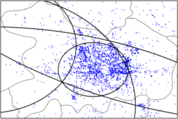
An example of narrowed region using CBG
-
2.
Static inactive hosts. Devices that are visible by few protocols (ICMP, BGP, etc.) such as routers, firewalls. These hosts are stable but hard to find. Only few of them have host names that have finer granularity than city-level.
-
3.
Unreachable hosts. Devices that are frequently off-line or invisible to ICMP.

In the narrowed region containing target host T, one needs to traceroute all landmarks in L and record paths. Figure 2 illustrates the network measurement procedure. Paths between vantage points (solid squares, V1 and V2) and landmarks (empty squares) are denoted as solid lines, and those with unreachable routers are denoted as dotted lines. In Fig. 2, (L1,L2,L3,L4,L5) are five landmarks sampled in target region. ICMP packages are transferred through routers and paths are split from four intermediate routers, (R1,R2,R3,R4). We ignore other routers because they only occur once in all paths, so that we cannot get more information. We denote paths split from these routers as relative paths, e.g. Pth(L3,R4,L4).

Controlling vantage points to discover intermediate routers
SLG purely pins target host to the landmark with the minimum relative latency, because geographical constraints are loose in narrowed region. Therefore, the results are dependent on the distribution of landmarks. As mentioned in previous section, most landmarks collected from web servers tend to be self-clustered and close to active hosts. It is obvious in Fig. 3 that the number of landmarks in two circles are both 7. However, radiuses of them are 2 and 0.3 km, which means that the landmark density in the smaller circle is 44 times larger than that of the larger one. This implies that host in large circle may be located with average error of 2 km which is 7 times larger than that in the smaller one.

Landmarks collected from websites
This paper is going to solve these two problems:
-
1.
Algorithms based on long distance calculation cannot get more accurate results since there is no more details about fine-grained information of the network. Therefore, distance estimation method within localized region needs to be studied.
-
2.
Geolocation accuracy is heavily depended on both vantage points and passive landmark distributions. Most of the time, vantage points are far away from target host because their locations are fixed. An algorithm that is independent to the distribution of vantage points and the density of passive landmarks is needed.
Geolocation model
We first narrow the confidence region of the target with coarse-grained geolocation method inspired by CBG and SLG. Based on traceroute data collected from landmarks in this region, we mine frequently occurred routers in all paths. In theory, if there is a router in more than three paths, it can be located by passive landmarks. As intermediate routers are usually closer to landmarks than vantage points, these routers are precisely located with the following algorithm.
Feature selection
Previous methods choose network latencies as geographical distance constraints. However, in the narrowed region, geographical distance constraints are loose. Therefore, we use both latencies (RTT) and hop counts (N) as network environment constraints. Denote the set of intermediate routers as R={Rm∣m∈[0,M]}, vantage points as V={Vk∣k∈[0,K]} and landmarks as L={Li∣i∈[0,I]}, where M, K, I are the amounts of routers, vantage points and landmarks. For each pair of intermediate router Rm and path Pth(Vk,Li), we calculate latency and hop count
Distance estimation maps measurement data to geographical distance. To find the best distance estimation algorithm in the narrowed region, we use three different ways to convert network constraints to geographical constraints.
Linear estimation
As network environment is bound to its geographical region, we assume that the inflated latency is small. Therefore the geographical distance between two nodes is partially proportional to the propagation delay. Geolocation methods usually measure the total delay (RTT) because propagation delay cannot be directly measured. We ignore detailed topologies among common routers and end nodes and represent them by N-term. The reason is that other delays (processing delay, queuing delay, transmission delay, etc.) are positively correlated to the number of intermediate nodes.
Denote latency and hop count between intermediate router Rm and landmark Li as RTTmi and Nmi, then linear estimated distance between two nodes can be presented as:
We train coefficients θ(θ0,θ1,θ2) with all relative paths between landmarks. Denote landmarks as L={L1,L2,…,Ln}, vantage points as V={V1,V2,…,Vm}. For each pair of landmarks Li,Lj∈L (with correlated vantage point Vk∈V), we use relative delay rRTTij and hop count rNij between Li and Lj:
as training data, use L1 distance:
as loss function. Where Rij, gij, dij denotes the common router, estimated distance and geographical distance between Li and Lj. We can describe the feature of network in this region with existing linear regression methods (e.g. gradient descent algorithm, least square regression).
Non-linear estimation
Noticing that hop counts between landmarks in moderately connected Internet are usually large, we filter out paths that are above the thresold of hop count. The choice of threshold varies with different network environments. Another solution is statistical estimation. We still use dij as training data, (rRTTij,rNij) as training features and L1 as loss function. Instead of linear regression, we use truncated normal distribution:
as the kernel function to estimate geographical distance with maximum likelihood probability, where Φ(μ/σ) is the cumulative distribution function of normal distribution. We choose normal distribution because it is well defined. We also use gamma distribution:
as the kernel function to get a more general result.
Maximum likelihood estimation
As shown in Fig. 4, we use maximum likelihood estimation with landmarks to geolocate target router Rm. Likelihood function depends on distance estimation method. The main purpose of maximum likelihood estimation is to find a point \((x^{\prime }, y^{\prime })\) that maximize target likelihood function. Assuming that we have K landmarks with geographical locations (x1,y1),(x2,y2),…,(xK,yK), when locating an intermediate router, we search landmarks that connect to it. Denote them as (Lm1,Lm2,…,Lmk).

Reverse locate intermediate router by landmarks
Linear estimation. Geographical distances can be calculated by coefficient θ trained before. Maximum likelihood results meet the following equations:
Great circle distance gij is written as
With this prerequisite, we can simplify Eq. 7
Note that geographical distance between two point doesn’t precisely meet Eq. 9 unless they are close to each other. Our algorithm is localized so that this approximation is acceptable. We can reduce Eq. 9 to a linear function
where
and
The least square estimation of X can be easily calculated by
Non-linear estimation. As discussed before, linear estimation loses network structure. We use log likelihood function
Target location xm is the point that maximize the likelihood function
Location target host
Previous works usually focus on geolocating target host, while the fact is that intermediate routers are usually more stable than end hosts. As long as we locate these routers, we can easily find the nearest intermediate router which is usually closer than other landmarks. As shown in Fig. 5, when geolocating reachable target T or unreachable host U, we find the nearest router by searching traceroute data without any further calculation.

Geolocate target host based on intermediate routers
Analysis
Portion of intermediate routers
The theoretical support of our method is that we can find a considerable portion of intermediate routers compared to the amount of passive landmarks. For mesh network (most commonly used), we assume that the number of routers is large enough. To verify our assumptions, we sample 200 landmarks in Beijing. We use a vantage point located in Beijing and collect routes by traceroute. Figure 6 presents the portion of intermediate routers occurred in more than 3 paths. As shown in the figure, more than 20 routers were found among 200 landmarks. In this convention, we assume that the amount of secondary landmarks takes more than 10% of web based landmarks.

Portion of intermediate routers
Choice of training parameters
No matter linear or non-linear estimation, we both use relative latencies generated by passive landmarks instead of round-trip time from vantage points as training data. We think it is more reasonable than using vantage points, because vantage points are sparsely distributed at a large scale and usually far away from target. While landmarks are dense and close to the target, parameters trained by these measurements are more convincing and suitable to local environment. Though relative paths are more complex than direct paths, as long as we limit the hop count, the corresponding error is acceptable.
Compared to TBG and Octant
It is proved in TBG and Octant that introducing network topology into geolocation may achieve higher accuracy. TBG controls all vantage points to measure routes to target host. It takes each node in these routes as a variable. Distance constraints between these nodes can be represented by inequalities with transmission delays and dynamic errors. TBG minimizes the sum of errors by solving the existing math problem and the location of target host is therefore calculated. TBG relies on a global optimization that minimizes average location error for all nodes. This can introduce extra error when locating target host by reducing errors on those of intermediate routers. Octant also geolocates all nodes appeared in routes. It uses multilateration with vantage points to geolocate intermediate node. Once an intermediate node is geolocated, it’s used as another vantage point to geolocate the following nodes. There are some improvements of our methods:
-
1.
These methods cannot be accurate in most situations because of the restriction of vantage points. The situation is quite rare that we cannot depend our system on the unchanging vantage points. Even if we can find adequate vantage points in some situations, our method won’t perform worse. TBG and Octant calculate all routers’ location constraints in paths that takes more computation time and introduces more calculation error. To decouple measurement data from vantage points, we survey landmarks in target region and only choose routers that appear in more than three routes. These routers have higher information and are much closer to target host than vantage points.
-
2.
We use “reversed measurement” to locate these nodes. Both TBG and Octant use around 20 or more vantage points that are distributed at a large scale. However, Hu et al. (2012) have proved that geolocation results is heavily dependent on the distribution of vantage points. Long distance latency measurement will introduce large positioning error. The problem can be revealed by the long tails of graphs of existing methods. While our “reversed measurement” take landmarks as vantage points to geolocate intermediate nodes with multilateration. In this way, we manage to perform topology discovery independent to the distribution of vantage points. We also reduce the geolocation errors in regions that are lack of passive landmarks.
Our method works without the constraints from the locations of vantage points and the densities of passive landmarks. It manages to improve existing topology-based methods. It may introduce more time overhead because of the number of landmarks, but they can be solved by parallelization.
Datasets
We use web page crawler and POI data from online map service to find landmarks. We collect 3839 landmarks in Beijing and check their visibilities by ping. We get 1124 visible landmarks. In order to validate performances of our method on different landmark densities, we split the dataset into three subsets.
University dataset
Landmarks from scholar institutions are stable and precise (Klingaman et al. 2006). However, we find that nodes from PlanetLab are invisible in China. Therefore, we manually collect web servers of universities in Beijing because most universities host their web servers locally. We validate these landmarks with their RDAP information and mail server addresses and finally get 48 accurate university landmarks.
City dataset
City dataset consists of hotels, organizations and other web servers from online map service. While there are thousands of landmarks, we cannot validate all of them manually. Therefore, we access their websites using their IPs and domain names. If the contents returned by the two sources are the same, we confirm that the corresponding landmark is valid. After the validation, we collect 1079 city landmarks. To validate the performance on coarse-grained dataset, we randomly select a circular region with radius of 25 km and lower landmark density compared to common dataset. These landmarks constitute only around 5% of total landmarks.
Partition
We randomly choose 30% of each dataset as test dataset to evaluate accuracy improvement. We analyze accuracy improvement of our method especially in localized region (with sparsely distributed landmarks).
Performance evaluation
We perform our experiments on datasets mentioned in previous section. As described in Fig. 3, we will prove that our method manage to solve this problem.
Traceroute is conducted to collect paths from vantage points to 699 landmarks. We study conditional probability distribution of geographical distance with given round-trip time latency and hop count. As shown in Fig. 7, the conditional probability distribution is approximately gamma distribution.

Conditional probability distribution of geographical distance given RTT and N
Gamma distribution can be converted to normal distribution when α is high. In consideration of computational complexity, we take normal distribution as the kernel function.
University dataset
Firstly, we conduct the experiment on university dataset. 13 (30%) landmarks are randomly chosen as test data and the rest 35 are training data. We measure relative paths and delays between target and landmarks with traceroute. Examples of measurement data are shown in Table 1. We find common routers in these paths to help geolocate target. One example is shown in Table 2, it’s connected by 2 landmarks (219.239.107.9 and 210.75.250.212). We manage to geolocate 7 common routers with the test set, which means we can extend our available landmarks by 20%.
To evaluate the efficiency of our method, we compare the geolocation errors to SLG, one of the latest geolocation methods. Figure 8 compares the cumulative distribution of the proposed common router-based geolocation (CRG) and SLG, shown by solid curve and dashed curve respectively. As shown in Fig. 8, the largest geolocation error of the proposed algorithm is 18 km, but for SLG, the number is 37 km. The details are listed in Table 3. There are about 25% of geolocation results require common routers as landmarks. Especially, when using common routers as secondary landmarks, the results are significantly more accurate than those of SLG. We evaluate the proposed algorithm by cross-validation because the amount of university landmarks is too small. The results show that we manage to reduce error of geolocation by about 10% compared to SLG.

Cumulative distribution of geolocation error of CRG and SLG
City dataset
We find 492 intermediate routers that appear in at least three paths. They constitute around 70.43% of the amount of landmarks. We denote these routers by upside-down triangle and plot then on Fig. 9. Dotted circle in Fig. 9 shows the narrowed confidence region after we take intermediate routers into consideration. We manage to reduce error radius by about 25% (from 2 to 1.5 km) in the larger circle. Figure 9 also implies that our method performs better when landmarks are sparsely distributed.

Landmarks with intermediate routers
We perform the same experiment on city dataset and the 5% one. As shown in Fig. 10, though the median error distance of these methods are similar, the largest error distance of CRG is 31 km and that of SLG is more than 45 km. This means that convergence speed of CRG is faster than SLG. It meets our expectation that the proposed method performs better in regions with sparsely distributed landmarks.

Comparison of cumulative probability of SLG, CRG and CRG with linear estimation in 5% dataset
Eventually, a city-level experiment is performed and the comparison of cumulative probability is shown in Fig. 11. The proposed method still performs better than SLG at the rate of convergence.

Comparison of cumulative probability of SLG, CRG at city level
Overall, average positioning error on city dataset is larger than that on university dataset, which is reasonable.
Result analysis
In general, the proposed method gets the best result on university dataset with the median error distance of 9 km and the largest error distance of 18 km. City-level result performs the worst. As shown in Table 3, we manage to reduce geolocation errors for most of the targets, except for some nodes, such as 124.42.73.141. The reason is that our method prefers intermediate routers. SLG has proved its efficiency when there’re fine-grained landmarks and well-connected network, while our method covers the opposite situation. Node 124.42.73.141 has a nearby landmark while our method chooses to geolocate it with the closest router. However, we find that there’s no nearby intermediate routers around this node in Table 3. Therefore, our method introduces higher geolocation error in this situation. We cannot always find a closer node than a nearby landmark especially in area with moderately connected network and fine-grained landmark density (similar to situation of L3 and L4 simulated in Fig. 2). However, most of them need intermediate routers to fix the lack of landmarks. Note that university dataset is sparsely distributed in the city, our method is more suitable in this situation.
Above conclusion implies that the lower landmark density of target region, the better results our method can achieve. The results prove our approach suitable for situations that existing methods cannot handle. Though our method doesn’t perform better with fine-grained landmarks (most of them are close to each other in city dataset in Fig. 3), we cannot always find sufficient landmarks especially in well protected regions.
Security concerns
Geolocation security is the foundation of physical security. It’s important to geolocate target host when we are attacking or been attacked. However, IP Geolocation is hard to detect. There is still no real-time geolocation method with feasible results. Public and commercial geolocation services provide real-time results, so they are most commonly used. However, geolocation accuracies of these services are not acceptable (Gharaibeh et al. 2017).
To achieve higher accuracy and lower response delay, geolocation results based on measurements and data mining are used as caches. They are conducted at preparation phase. One must keep itself from delay-based measurements and information exposure at any time in order to protect itself from being located. While common delay-based measurements are simple and benign, it is hard to detect. Delay-based measurements can be evaded by long distance dialup, proxy servers, remote sessions, etc (Muir and Oorschot 2009). It’s also possible to attack geolocation system by manipulating network delays and hops (Gill et al. 2010). Our method focuses on the limit of information exposure. Lack of landmarks may be caused by protection (which is a security problem) or the functional area that target host lies in. Our method proposes distributed nodes around the target, so that network manipulations (Gill et al. 2010) won’t influence our method unless it takes control of all routers to landmarks in the area. As shown in the experiment results, our method manages to improve the geolocation accuracy despite the lack of landmarks.
Conclusion
Towards existing problem that geolocation result is heavily dependent on landmark density and vantage point position, a novel IP geolocation method based on discovering intermediate routers as secondary landmarks is presented in this paper. The proposed method takes advantage of passive landmarks to perform topology measurements without the limitation of the distribution of vantage points. It finds frequently appeared common routers. Most of them can be geolocated by existing landmarks and routes. These common routers have more information than other nodes. The proposed method chooses these routers as secondary landmarks to help increase landmark density. This method works well in regions with sparsely distributed landmarks. We have evaluated our method in Beijing on university and city dataset with different landmark densities. Experimental results show that we manage to reduce long tail effect on all datasets, especially on university dataset by about 50%.
Our work manages to decouple geolocation result from vantage points and landmark densities. The proposed method can be further improved by replacing maximum likelihood estimation to other methods that take network structures into consideration.
References
Archipelago (2007) Archipelago measurement infranstructure. http://www.caida.org/projects/ark/. Accessed Sept 2018.
Eriksson, B, Barford P, Sommers J, Nowak R (2010) A learning-based approach for IP geolocation. In: Krishnamurthy A Plattner B (eds)Passive and Active Measurement. PAM 2010. Lecture Notes in Computer Science, vol 6032.. Springer, Berlin.
Gharaibeh, M, Shah A, Huffaker B, Zhang H, Ensafi R, Papadopoulos C (2017) A Look at Router Geolocation in Public and Commercial Databases In: proceedings of the 2017 Internet Measurement Conference, London.
Gill, P, Ganjali Y, Wong B, Lie D (2010) Dude, where’s that ip?: Circumventing measurement-based ip geolocation In: Proceedings of the 19th USENIX Conference on Security, USENIX Association, 16–16.. USENIX Security’10, Berkeley. http://dl.acm.org/citation.cfm?id=1929820.1929842.
Gueye, B, Ziviani A, Crovella M, Fdida S (2006) Constraint-based geolocation of Internet hosts. IEEE/ACM Trans Networking 14(6):1219–1232.
Guo, C, Liu Y, Shen W, Wang HJ, Yu Q, Zhang Y (2009) Mining the web and the Internet for accurate IP address geolocations In: IEEE INFOCOM 2009, 2841–2845.. IEEE, Rio de Janeiro.
Hanemann, A, Boote JW, Boyd EL, Durand J, Kudarimoti L, Łapacz R, Swany DM, Trocha S, Zurawski J (2005) Perfsonar: A service oriented architecture for multi-domain network monitoring. In: Benatallah B, Casati F, Traverso P (eds)Service-Oriented Computing - ICSOC 2005, 241–254.. Springer Berlin Heidelberg, Berlin, Heidelberg.
Heidemann, J, Pradkin Y, Govindan R, Papadopoulos C, Bartlett G, Bannister J (2008) Census and Survey of the Visible Internet In: Proceedings of the 8th ACM SIGCOMM Conference on Internet Measurement, 169–182.. ACM, New York. IMC ’08, https://doi.org/10.1145/1452520.1452542.
Hu, Z, Heidemann J, Pradkin Y (2012) Towards Geolocation of Millions of IP Addresses In: Proceedings of the 2012 Internet Measurement Conference, 123–130.. ACM, New York. IMC ’12, https://doi.org/10.1145/2398776.2398790.
Huffaker, B, Fomenkov M, Claffy k (2014) DRoP:DNS-based Router Positioning. ACM SIGCOMM Comput Commun Rev (CCR) 44(3):6–13.
Katz-Bassett, E, John JP, Krishnamurthy A, Wetherall D, Anderson T, Chawathe Y (2006) Towards IP geolocation using delay and topology measurements In: Proceedings of the 6th ACM SIGCOMM conference on Internet measurement (IMC ’06), 71–84.. ACM, New York.
Klingaman, A, Huang M, Muir S, Peterson L (2006) PlanetLab Core Specification 4.0. Tech. Rep. PDN–06–032, PlanetLab Consortium.
Laki, S, Mátray P, Hága P, Sebȯk T, Csabai I, Vattay G (2011) Spotter: A model based active geolocation service In: INFOCOM, 2011 Proceedings IEEE, 3173–3181.. IEEE, Shanghai.
Li, D, Chen J, Guo C, Liu Y, Zhang J, Zhang Z, Zhang Y (2013) IP-geolocation mapping for moderately connected Internet regions. IEEE Trans Parallel Distrib Syst 24(2):381–391.
Liu, H, Zhang Y, Zhou Y, Zhang D, Fu X, Ramakrishnan KK (2014) Mining checkins from location-sharing services for client-independent IP geolocation In: IEEE INFOCOM 2014 - IEEE Conference on Computer Communications, 619–627. https://doi.org/10.1109/INFOCOM.2014.6847987.
Matthews, W, Cottrell L (2000) The pinger project: active internet performance monitoring for the henp community. IEEE Commun Mag 38(5):130–136. https://doi.org/10.1109/35.841837.
Meyer, D, et al. (2005) University of oregon route views project. http://routeviews.org/. Accessed Sept 2018.
Muir, JA, Oorschot PCV (2009) Internet geolocation: Evasion and counterevasion. Acm Comput Surv (CSUR) 42(1):4.
Newton, A, Ellacott B, Kong N (2015) Http usage in the registration data access protocol (rdap). Internet Requests Comments. https://tools.ietf.org/html/rfc7480. Accessed Sept 2018.
Padmanabhan, VN, Subramanian L (2001) An investigation of geographic mapping techniques for Internet hosts, Vol. 31. ACM.
Route Server (2009) Public router servers. http://routeserver.org/.
Wang, Y, Burgener D, Flores M, Kuzmanovic A, Huang C (2011) Towards street-level client-independent IP geolocation, Vol. 11.
Weinberg, Z, Cho S, Christin N, Sekar V, Gill P (2018) How to catch when proxies lie: Verifying the physical locations of network proxies with active geolocation In: Proceedings of the Internet Measurement Conference, 203–217.. ACM, New York. IMC ’18, https://doi.org/10.1145/3278532.3278551, http://doi.acm.org/10.1145/3278532.3278551.
Wong, B, Stoyanov I, Sirer EG (2007) Octant: A comprehensive framework for the geolocalization of Internet hosts In: Proceedings of the 4th USENIX Symposium on Networked Systems Design & Implementation,(NSDI 07).. USENIX Association, Cambridge. https://www.usenix.org/conference/nsdi-07/octant-comprehensive-framework-geolocalization-internet-hosts.
Youn, I, Mark BL, Richards D (2009) Statistical geolocation of Internet hosts In: Proceedings of 18th Internatonal Conference on Computer Communications and Networks, 2009. ICCCN 2009, 1–6.. IEEE, San Francisco.
Acknowledgements
Not applicable.
Funding
Not applicable.
Availability of data and materials
To respect location privacy, the datasets collected from web to support the conclusions of this article are not available.
Author information
Authors and Affiliations
Contributions
All authors read and approved the final manuscript.
Corresponding author
Ethics declarations
Competing interests
The authors declare that they have no competing interests.
Publisher’s Note
Springer Nature remains neutral with regard to jurisdictional claims in published maps and institutional affiliations.
Rights and permissions
Open Access This article is distributed under the terms of the Creative Commons Attribution 4.0 International License(http://creativecommons.org/licenses/by/4.0/), which permits unrestricted use, distribution, and reproduction in any medium, provided you give appropriate credit to the original author(s) and the source, provide a link to the Creative Commons license, and indicate if changes were made.
About this article

Cite this article
Wang, Z., Li, H., Li, Q. et al. Towards IP geolocation with intermediate routers based on topology discovery. Cybersecur 2, 13 (2019). https://doi.org/10.1186/s42400-019-0030-2
Received:
Accepted:
Published:
DOI: https://doi.org/10.1186/s42400-019-0030-2