A framework for the extended evaluation of ABAC policies

Abstract

A main challenge of attribute-based access control (ABAC) is the handling of missing information. Several studies have shown that the way standard ABAC mechanisms, e.g. based on XACML, handle missing information is flawed, making ABAC policies vulnerable to attribute-hiding attacks. Recent work has addressed the problem of missing information in ABAC by introducing the notion of extended evaluation, where the evaluation of a query considers all queries that can be obtained by extending the initial query. This method counters attribute-hiding attacks, but a naïve implementation is intractable, as it requires an evaluation of the whole query space. In this paper, we present a framework for the extended evaluation of ABAC policies. The framework relies on Binary Decision Diagram (BDDs) data structures for the efficient computation of the extended evaluation of ABAC policies. We also introduce the notion of query constraints and attribute value power to avoid evaluating queries that do not represent a valid state of the system and to identify which attribute values should be considered in the computation of the extended evaluation, respectively. We illustrate our framework using three real-world policies, which would be intractable with the original method but which are analyzed in seconds using our framework.

Introduction

Attribute-Based Access Control (ABAC) is emerging as the de facto paradigm for the specification and enforcement of access control policies. In ABAC, policies and access requests are defined in terms of attribute name-value pairs. This provides an expressive, flexible and scalable paradigm that is able to capture and manage authorizations in complex environments.

Although ABAC provides a powerful paradigm for access control, ABAC systems require that all the information necessary for policy evaluation is available to the policy decision point, which might be difficult to achieve in modern systems. Recent years have seen the emergence of authorization mechanisms that go beyond the view of a centralized monitor with full knowledge of the system. Authorization mechanisms increasingly rely on external services to gather the information necessary for access decision making (e.g., Amazon Web Services rely on third-party identity providers and federated identity systems, the OAuth 2.0 protocol enables delegation of authorization). The use of external information sources for attribute retrieval makes it difficult to guarantee and, in some cases, even to check that all necessary information has been provided. Moreover, in some domains like IoT, it might be difficult and costly to gather (accurate) information needed for policy evaluation. Missing information can significantly influence query evaluation and pose significant risks to a large range of modern systems.

To this end, existing ABAC models are often equipped with mechanisms to handle missing attributes during policy evaluation.

However, these mechanisms have some intrinsic drawbacks (Crampton and Huth 2010; Tschantz and Krishnamurthi 2006). For instance, eXtensible Access Control Markup Language (XACML) (OASIS 2013), the de facto standard for the specification and evaluation of ABAC policies, provides a mechanism to deal with missing attributes. However, Crampton et al. (2015) showed that the evaluation of a XACML query can yield a decision that does not necessarily provide an intuitive interpretation on whether access should be granted or not due to the fact that some information needed for the evaluation might be missing. These drawbacks make the evaluation of ABAC policies vulnerable to attribute hiding attacks where users can obtain a more favorable decision by hiding some of their attributes (Crampton and Morisset 2012).

To make the evaluation of ABAC policies robust against attribute hiding attacks, previous work (Crampton et al. 2015) has proposed a novel approach that allows for an extended evaluation of ABAC policies.

In a nutshell, the authors suggest that the evaluation of a given query is calculated using the evaluation of all queries that can be constructed from the initial query. This way, the extended evaluation unveils the risks when information could be, intentionally or not, hidden to the policy decision point. However, this approach requires exploring the state space for all possible queries, which is exponential in the number of attribute values, and therefore not particularly efficient.

In this work, we present a formal framework for the extended evaluation of ABAC policies that addresses this drawback, extending our previous work (Morisset et al. 2018). Our framework includes several evaluation methods, as well as the notions of query constraint, which is used to exclude those queries that are not possible within the system from the query space. Our framework relies on binary decision diagram (BDD)-based data structures for the encoding ABAC policies. As shown in previous work (Bahrak et al. 2010; Fisler et al. 2005; Hu et al. 2013), these data structures provide a compact encoding for storing the decisions yielded by an ABAC policy for every query and for efficient policy evaluation. Moreover, the framework is equipped with an efficient method to compute the extended evaluation directly on the BDD structure. To further optimize the computation of the extended evaluation, we also introduce the notion of attribute value power, which provides insights into the impact of attributes on decision making. This can help determine which attribute should be considered in the computation of the extended evaluation by excluding attribute values when they have no power (i.e., they have no impact on decision making). To the best of our knowledge, this is the first work that investigates the impact of attributes on the evaluation of ABAC policies.

We demonstrate our approach on three complex case studies, where a naïve approach would deal with a query space comprising several millions of states, whereas our approach compiles in a few seconds a compact decision diagram. Compared to Morisset et al. (2018), we also analyze the time required for policy evaluation using BDD data structures and we show that our framework outperforms SAT-based policy frameworks. Moreover, we present a quantitative analysis of the attribute value power for the three case studies.

The remainder of this paper is organized as follows. The next section presents preliminaries on ABAC and the notion of extended evaluation. “Problem statement” section introduces a motivating example and provides a formulation of the problem. “Query constraints” section presents the notion of query constraint. “Attribute power” section presents the notion of attribute value power.“Efficient extended evaluation computation” section presents a novel algorithm to compute the extended query evaluation. “Case studies” section provides a validation of our approach on three real-world policies. Finally, “Related work” section discusses related work and “Conclusion” section concludes the paper. We provide the proofs of the theorems in appendix.

Preliminaries

This section presents a general view of how Attribute-Based Access Control (ABAC) policies and queries are evaluated using PTaCL (Crampton and Morisset 2012), which provides an abstraction of the XACML standard (OASIS 2013). We first present the syntax of PTaCL, which encompasses two different languages: one for targets, which is used to decide the applicability of a policy to a query, and another for policies, which is used to specify how policies are combined together. We then present two evaluation functions proposed for PTaCL: the standard evaluation function, introduced in Crampton and Morisset (2012) and the extended evaluation function, introduced in Crampton et al. (2015).

ABAC syntax

In ABAC, queries and policies are defined in terms of attribute name-value pairs (instead of the traditional triple subject, object, access mode). More precisely, let $\mathcal {A} = \{a_{1}, \dots, a_{n}\}$ be a finite set of attributes, and given an attribute $a \in \mathcal {A}$, let $\mathcal {V}_{a}$ be the domain of a. The set of queries$Q_{\mathcal {A}}$ is then defined as $\wp \left (\bigcup _{i=1}^{n} a_{i} \times {\mathcal {V}}_{a_{i}}\right)$, and a query q={(a₁,v₁),…,(a_k,v_k)} is a set of attribute name-value pairs (a_i,v_i) such that $a_{i}\in \mathcal {A}$ and $v_{i}\in \mathcal {V}_{a_{i}}$. A query encompasses both a specific request for access, and a current view of the world describing the different entities concerned by that request.

The PTaCL language is tree-based, i.e. policies are recursively constructed from atomic policies using operators. This vision follows the traditional “separation of concerns” principle: each policy might regulate accesses to a specific sub-domain of an organization, or regulate accesses done by a specific category of users or in specific contexts. In order to identify which policies are applicable to which targets, PTaCL introduce a target language $\mathcal {T}_{\mathcal {A}}$, such that a target $t \in \mathcal {T}_{\mathcal {A}}$ is defined as:

$$ t=(a, v)\mid \mathsf{op}(t_{1}, \dots, t_{n}) $$

where (a, v) is an attribute name-value pair and op is an n-ary operator defined over the set $\mathcal {D}_{3} = \{1, 0, \bot \}$, indicating that the target matches the query, that the target does not match the query, and that it is indeterminate whether the target matches the query or not (the semantical evaluation of targets is described below). Table 1 presents the operators provided by PTaCL as well as operators commonly used in ABAC languages. It is worth noting that the set of operators { ¬,E₁, } is canonically complete (Crampton and Williams 2016), i.e. any 3-valued operator can be constructed using these three operators.

Table 1 Operators on the set $\mathcal {D}_{3} = \{1,0,\bot \}$

PTaCL also defines a policy language $\mathcal {P}_{\mathcal {A}}$, where a policy $p \in \mathcal {P}_{\mathcal {A}}$ is defined as:

$$p= 1 \mid 0 \mid (t, p) \mid \mathsf{op}(p_{1}, \dots, p_{n}) $$

where 1 and 0 represent the allow and deny decisions respectively, (t, p) is a target policy and op is an n-ary operator, also defined on the three-valued set {1,0,⊥}, where ⊥ represents the not-applicable decision. Although this set is syntactically equivalent to the one used for targets, the meaning of the values in the set depends on whether it is used as a target or as a policy. This should always be clear from the context in the remainder of this paper.

ABAC evaluation

Given the set of policies $\mathcal {P}_{\mathcal {A}}$, the set of queries $Q_{\mathcal {A}}$ and a set of decisions $\mathcal {D}$, an evaluation function is a function $\llbracket \cdot \rrbracket : \mathcal {P}_{\mathcal {A}} \times Q_{\mathcal {A}} \rightarrow \mathcal {D}$ such that, given a query q and a policy p, ⟦p⟧(q) represents the decision of evaluating p against q. PTaCL has two main policy evaluation functions, which handle missing attributes in a different way. For the sake of uniformity, hereafter we might use different notations than those used in the original publications.

Standard evaluation

The standard evaluation consists in evaluating a target to ⊥ when the attribute is completely missing from the query, to 0 if the attribute is present in the query, but without the appropriate value, and to 1 otherwise. A policy then evaluates to a set of decisions within $\mathcal {D}_{7}=\wp (\{1,0,\bot \}) \backslash \emptyset$ where 1 and 0 indicate that access should be granted or denied respectively, and ⊥ that the policy is not applicable to a given query.

Non-singleton decisions are returned when the query does not provide the information necessary to evaluate a target (i.e., the target evaluates to ⊥). Intuitively, non-singleton decisions correspond to the indeterminate decision in XACML (Morisset and Zannone 2014).

More formally, the semantics of a target t is given by the function:

$$\begin{array}{*{20}l} \llbracket \cdot \rrbracket_{\mathrm{T}} & : \mathcal{T}_{\mathcal{A}} \times Q_{\mathcal{A}} \rightarrow \mathcal{D}_{3}\\ \llbracket (a,v) \rrbracket_{\mathrm{T}} (q) & = \left\{ \begin{array}{ll} 1 & \text{if \((a,v) \in q\)} \\ \bot & \text{if} \; \forall v^{\prime}\in \mathcal{V}_{a}: \left(a,v^{\prime}\right) \not\in q\\ 0 & \text{otherwise} \end{array}\right.\\ \llbracket \mathsf{op}(t_{1}, \dots, t_{n}) \rrbracket_{\mathrm{T}} (q) & = \mathsf{op}\left(\llbracket t_{1} \rrbracket_{\mathrm{T}} (q), \dots, \llbracket t_{n} \rrbracket_{\mathrm{T}} (q) \right) \end{array} $$

The standard semantics of a policy p is given by the function:

$$\begin{array}{*{20}l} \llbracket \cdot \rrbracket_{\mathrm{P}} & : \mathcal{P}_{\mathcal{A}} \times Q_{\mathcal{A}} \rightarrow \mathcal{D}_{7} \\ \llbracket 1 \rrbracket_{\mathrm{P}} (q) & = \{1\}\\ \llbracket 0 \rrbracket_{\mathrm{P}} (q) & =\{0\}\\ \llbracket (t, p) \rrbracket_{\mathrm{P}} (q) & = \left\{ \begin{array}{ll} \llbracket p \rrbracket_{\mathrm{P}} (q) & \text{if} \; \llbracket t \rrbracket_{\mathrm{T}} (q) = 1 \\ \{\bot\} & \text{if} \; \llbracket t \rrbracket_{\mathrm{T}} (q) = 0 \\ \{\bot\} \cup \llbracket p \rrbracket_{\mathrm{P}} (q) & \text{otherwise} \end{array}\right.\\ \llbracket \mathsf{op}(p_{1}, \dots, p_{n}) \rrbracket_{\mathrm{P}} (q) & = \mathsf{op}^{\uparrow} \left(\llbracket p_{1} \rrbracket_{\mathrm{P}} (q), \dots, \llbracket p_{n} \rrbracket_{\mathrm{P}} (q)\right) \end{array} $$

where, given an operator $\mathsf {op} : \mathcal {D}_{3}\times \mathcal {D}_{3} \to \mathcal {D}_{3}$ and any non-empty sets $X, Y \subseteq \mathcal {D}_{3}$, $\mathsf {op}^{\uparrow } : \mathcal {D}_{7}\times \mathcal {D}_{7} \rightarrow \mathcal {D}_{7}$ is defined as op^↑(X,Y)={op(x,y)∣x∈X∧y∈Y}. Intuitively, op^↑ corresponds to operator op extended in a point-wise way to sets of decisions.

Extended evaluation

The extended evaluation relies on a non-deterministic attribute retrieval (Crampton et al. 2015)¹. The fundamental intuition is to model the fact that a query might represent a partial view of the world, whereby some attribute values are missing.

The extended evaluation of an ABAC policy is computed using two functions: the simplified evaluation function and the extended evaluation function. The simplified evaluation function ⟦·⟧ ignores missing attributes,² and therefore always returns a single decision. Formally:

$$\begin{array}{*{20}l} \llbracket \cdot \rrbracket_{\mathrm{B}} & : \mathcal{P}_{\mathcal{A}} \times Q_{\mathcal{A}} \to \mathcal{D}_{3} \\ \llbracket 1 \rrbracket_{\mathrm{B}} (q) & = 1\\ \llbracket 0 \rrbracket_{\mathrm{B}} (q) & = 0\\ \llbracket (t, p) \rrbracket_{\mathrm{B}} (q) & = \left\{ \begin{array}{ll} \llbracket p \rrbracket_{\mathrm{B}} (q) & \text{if} \; \llbracket t \rrbracket_{\mathrm{T}} (q) = 1 \\ \bot & \text{otherwise} \\ \end{array} \right.\\ \llbracket \mathsf{op}(p_{1}, \dots, p_{n}) \rrbracket_{\mathrm{B}} (q) & = \mathsf{op}(\llbracket p_{1} \rrbracket_{\mathrm{B}} (q), \dots, \llbracket p_{n} \rrbracket_{\mathrm{B}} (q)) \end{array} $$

The extended evaluation function evaluates a query to all possible decisions that can be obtained by adding possibly missing attributes. Hereafter, we represent a query space as a directed acyclic graph (save for self-loops) $(Q_{\mathcal {A}}, \rightarrow)$, where $Q_{\mathcal {A}}$ is a set of queries, and $\rightarrow \subseteq Q_{\mathcal {A}} \times Q_{\mathcal {A}}$ is a relation such that, given two queries $q,q^{\prime }\in Q_{\mathcal {A}}$, q→q^′ if and only if q^′=q∪{(a,v)} for some attribute $a\in \mathcal {A}$ and some value $v \in \mathcal {A}$.

Note that some extensions of a query q may not be possible. For instance, for a given Boolean attribute, it might not make sense to have in the same query both true and false for that attribute. Hence, Crampton et al. introduce in Crampton et al. (2015) the notion of negative attribute value to explicitly indicate that an attribute cannot have a certain value in a given context and the notion of well-formed predicate $\mathsf {wf} : Q_{\mathcal {A}} \rightarrow \mathbb {B}$ over queries to ensure that a query does not contain both an attribute value and its negation.

Based on these notions, the extended evaluation function ⟦·⟧_E is defined as follows:

$$\begin{array}{*{20}l} \llbracket \cdot \rrbracket_{\mathrm{E}} & : \mathcal{P}_{\mathcal{A}} \times Q_{\mathcal{A}} \to \mathcal{D}_{8} = \wp(\{1, 0, \bot\}) \\ \llbracket p \rrbracket_{\mathrm{E}} (q) & = \left\{ \llbracket p \rrbracket_{\mathrm{B}} \left(q^{\prime} \right) \mid q \rightarrow^{*} q^{\prime} \land \mathsf{wf}(q^{\prime}) \right\} \end{array} $$

where →^∗ denotes the reflexive-transitive closure of →. With the restrictions imposed on →, the relation →^∗ reduces to the subset relation on queries. It is worth observing that ⟦·⟧_E returns the empty set for any query that does not satisfy wf. In “Query constraints” section we will refine predicate wf by introducing the notion of query constraint to capture more complex domain requirements.

Problem statement

We illustrate the drawbacks of the standard and extended evaluation functions through a sample policy. Consider a system wherein access is based on the nationality of users. In particular, the system allows Belgians to access system resources, whereas the Dutch are not. This policy can be represented as follows:

$$p = (({\mathbf{nat}}, \mathsf{BE}), 1) \bigtriangleup (({\mathbf{nat}}, \mathsf{NL}),0) $$

Standard evaluation function⟦·⟧_P: Crampton et al. (2015) have shown that the standard evaluation, which is the one used by XACML, can yield a decision that does not necessarily provide an intuitive interpretation on whether access should be granted or not due to the fact that some information needed for the evaluation might be missing. In other words, given a policy, it is possible for a query to evaluate to a set of decisions D such that there exists a decision d∈D for which the query extended with additional attribute values would not evaluate to d, while there could be some decision d^′∉D for which the query extended with some additional attribute values would evaluate to d^′. We exemplify these issues in the following example.

Consider a user submitting the query q={(nat,BE)}, stating that the user is Belgian. This query evaluates ⟦p⟧_P({(nat,BE)})={1}, i.e. the access is granted. However, it is possible for a user to have multiple nationalities, and in some cases, it might be possible for a user to hide some nationalities³. In our case, the user might be hiding that she also has a Dutch nationality, in which case the access should have been denied since ⟦p⟧_P({(nat,BE),(nat,NL)})={0}.

Extended evaluation function⟦·⟧_E: To overcome the drawbacks of function ⟦·⟧_P, given a policy p and a query q, a policy enforcement point (i.e., the point in the system in charge of enabling an access query or not) can evaluate ⟦p⟧_E(q) in addition to ⟦p⟧_B(q), to determine whether any missing attribute could change the evaluation. In particular, we obtain ⟦p⟦_E({(nat,BE)})={1,0} indicating that there exists a query (i.e., a view of the world) reachable from q that should be denied.

Computing ⟦p⟧_E(q), however, requires evaluating all queries that can be constructed from the initial query q. This leads to two main problems:

• A naïve implementation of ⟦·⟧_E requires exploring a very large query space, making policy evaluation inefficient.

• Not all queries that can be constructed from the initial query might be a plausible view of the world. The evaluation of those queries can lead to misleading decisions.

To visually represent these problems, consider (the portion of) the query space in Fig. 1, which is explored in the evaluation of query q. In the figure, nodes represent queries (with q₀ the empty query) and edges are annotated with a label indicating how a query has been extended, i.e. q_iNL→q_j denotes q_j=q_i∪{(nat,NL)}.

Fig. 1

Portion of the query space

Concerning the first problem, we have to account that there are 206 sovereign states recognized by the United Nations⁴, and users can have more than one nationality. Therefore, computing ⟦p⟧_E(q) requires evaluating 2²⁰⁵ queries (i.e., the queries that can be constructed from the initial query {(nat,BE)}), which is clearly infeasible.

More importantly, ignoring domain constraints can result in decisions that cannot be reached in practice, thus providing misleading information for decision making. We illustrate this using two examples.

Although there is no limit on the number of nationalities individuals can hold according to international laws, it is reasonable to assume that this number is limited. For the sake of exemplification, let us assume that individuals cannot hold more than three nationalities.

According to this domain constraint, no queries formed by four or more attribute name-value pairs are reachable from the initial state (i.e., queries q₁₂ to q₁₆ in Fig. 1) as they are not plausible views of the world. If those queries are evaluated, the access control system can return decision that cannot be reached in practice. For instance, consider q₁₀={(nat,BE),(nat,GB),(nat,FR)}. The (simplified) evaluation of q₁₀ against policy p returns a permit decision, i.e. ⟦p⟧_B(q₁₀)={1}. However, ignoring domain constraints, we have ⟦p⟧_E(q₁₀)={1,0}. In fact, the extended evaluation of q₁₀ requires evaluating q₁₅=q₁₀∪{(nat,NL)}, which however is not a plausible view of the system according to the domain requirement.

As another example, one can consider that several countries have constraints on double nationality. Suppose, for instance, that Austria does not allow dual nationality with the Netherlands⁵. In this case, we should exclude from the state space any query containing both attribute name-value pairs (nat,NL) and (nat,AT) (i.e., queries q₇, q₁₂, q₁₄ and q₁₆ in Fig. 1). Accordingly, given the query {(nat,AT)}, we expect this request to be never denied, even if some attribute is missing.

In contrast, if domain constraints are neglected, we obtain ⟦p⟧_E({(nat,AT)})={1,0,⊥}.

Contribution In the remainder of the paper, we will exploit these observations to establish the foundations for the design of practical policy frameworks supporting the extended evaluation of attribute-based access control policies. In particular:

• We introduce the notion of query constraint to identify which views of the world are plausible based on domain specific requirements and assumptions, thus constructing a realistic query space (“Query constraints” section).

• We introduce the notion of attribute value power to determine how much an attribute value is capable of triggering a specific decision (“Attribute power” section).

• We investigate practical approaches for the computation of the extended evaluation function ⟦·⟧_E (“Efficient extended evaluation computation” section).

Query constraints

A non-deterministic evaluation of ABAC policies requires the construction of all possible views of the world from a given query.

As shown above, many of these views may not be possible in practice. In fact, a system can be characterized by domain requirements and assumptions that determine which views of the world are plausible and which are not. The main problem lies in the fact that domain requirements and assumptions are typically defined outside the authorization mechanism and, thus, not available for policy evaluation.

It is worth emphasizing here that there is a fundamental distinction between queries that are not possible and queries that should be denied. In the previous section, a query including both Austrian and Dutch nationalities is neither denied nor granted, but considered instead as not possible.

To account for domain requirements within policy evaluation, we introduce the notion of query constraint. First, we present a language for the specification of query constraints and then we define a function for their evaluation.

Syntactically speaking, the language for constraints $\mathcal {C}_{\mathcal {A}}$ is such that a constraint $c \in \mathcal {C}_{\mathcal {A}}$ is defined as:

$$c= (a, v) \mid \mathsf{op}(c_{1}, \dots, c_{n}) $$

where (a,v) is an attribute name-value pair, and op is a Boolean operator. Intuitively, a query constraint is used to restrict the values that an attribute can assume in a query (hereafter we refer to this type of constraints as value constraints).

It is worth noting that the only difference between $\mathcal {C}_{\mathcal {A}}$ and $\mathcal {T}_{\mathcal {A}}$ (defined in “ABAC syntax” section) is that we do not consider three-valued operators for constraints. We therefore have $\mathcal {C}_{\mathcal {A}} \subseteq \mathcal {T}_{\mathcal {A}}$, since any Boolean operator trivially corresponds to a three-valued operator. The semantics of constraints is given by the following function:

$$\begin{array}{*{20}l} \llbracket \cdot \rrbracket_{\mathrm{C}} & : \mathcal{C}_{\mathcal{A}} \times Q_{\mathcal{A}} \rightarrow \mathbb{B} \\ \llbracket (a,v) \rrbracket_{\mathrm{C}} (q) & = \left\{ \begin{array}{ll} 1 & \text{if}\; (a,v) \in q \\ 0 & \text{otherwise} \end{array}\right.\\ \llbracket \mathsf{op}(t_{1}, \dots, t_{n}) \rrbracket_{\mathrm{C}} (q) & = \mathsf{op}(\llbracket t_{1} \rrbracket_{\mathrm{C}} (q), \dots, \llbracket t_{n} \rrbracket_{\mathrm{C}} (q)) \end{array} $$

We say that a constraint c is monotonic (resp. anti-monotonic) whenever, for every pair of queries $q,q^{\prime }\in Q_{\mathcal {A}}$ such that q⊆q^′, if ⟦c⟧_C(q)(resp. ⟦c⟧_C(q^′)) holds then ⟦c⟧_C(q^′) (resp. ⟦c⟧_C(q)) also holds.

Example 1

Some countries such as Singapore, Austria and India, do not allow dual nationality, leading to automatic loss of citizenship upon acquiring another nationality. Other countries restrict dual nationality to certain countries. For instance, Pakistan allows double nationality only with 16 countries and Spain allows only with certain Latin American countries, Andorra, Portugal, the Philippines and Equatorial Guinea. These requirements can be modeled using query constraints. For instance, the following constraint indicates that it is not possible to have both Austrian and Dutch citizenships: ¬((nat,AT)∧(nat,NL)).

Some constraints might be more complex to build. For instance, we might want to have cardinality constraints specifying the maximum number of values a particular attribute can take. However, there is no Boolean operator expressing directly such constraints. Instead, given an attribute a and a number k, we can generate the corresponding constraint enumerating all possible cases. We first write $\mathcal {A}_{\mid a} = \{ (a, v) \mid v \in \mathcal {V}_{a}\}$ for the set of all attribute name-value pairs for an attribute a. We then write $C_{a, k} = \left \{ s \subseteq \mathcal {A}_{\mid a} \mid \vert s \vert = k +1 \right \}$ for the set of subsets of $\mathcal {A}_{\mid a}$ with a cardinality equal to k+1. A cardinality constraint expressing that an attribute a can have at most k values can be expressed as:

$${card}_{a, k} = \bigwedge_{s \in C_{a, k}} \lnot \bigwedge_{(a, v) \in s} (a, v) $$

Any query containing more than k values for attribute a would have at least one set s∈C_a,k for which the conjunction of the attribute values would be true, rendering the whole conjunction card_{a, k} false.

Example 2

Consider the scenario in “Problem statement” section, such that, for the sake of exposition, we only consider six possible nationalities: FR, AT, GB, DE, BE and NL. The constraint that an individual cannot hold more than three nationalities can be expressed by the constraint card_nat,3, which consists of 30 conjunctions of conjunctions:

$$\begin{array}{*{20}l} {card}_{{\mathbf{nat}}, 3} = & \quad \lnot (({\mathbf{nat}}, \mathsf{FR})\land ({\mathbf{nat}}, \mathsf{AT}) \land ({\mathbf{nat}}, \mathsf{GB}) \land ({\mathbf{nat}}, \mathsf{DE})) \\ & \land \lnot (({\mathbf{nat}}, \mathsf{FR})\land ({\mathbf{nat}}, \mathsf{AT}) \land ({\mathbf{nat}}, \mathsf{GB}) \land ({\mathbf{nat}}, \mathsf{BE})) \\ & \land \dots \\ & \land \lnot (({\mathbf{nat}}, \mathsf{GB})\land ({\mathbf{nat}}, \mathsf{DE}) \land ({\mathbf{nat}}, \mathsf{BE}) \land ({\mathbf{nat}}, \mathsf{NL})) \end{array} $$

As demonstrated by the example above, the cardinality constraint for an attribute a can only be constructed in this form when the attribute domain $\mathcal {V}_{a}$ is finite. In this paper, our encoding of ABAC policies requires anyway finite domains for attributes, and we leave the investigation of infinite attribute domains for future work.

Hereafter, given a set of query constraints C, we write $Q_{\mathcal {A} \mid C}$ for the set $\left \{q \in Q_{\mathcal {A}} \mid \forall c \in C \,\, \llbracket c \rrbracket _{\mathrm {C}} (q)=1 \right \}$, and we consider for the definition of ⟦·⟧_E in “Extended evaluation” section that, given a query q, wf(q) if, and only if, $q \in Q_{\mathcal {A} \mid C}$.

Attribute power

In this section, we introduce the notion of attribute power, which, intuitively speaking, measures how often a given attribute is responsible for the policy to return a specific decision.

Our notion of power is inspired by the Banzhaf Power Index (1966), which was created in the context of electoral systems. While Banzhaf focused on the capability of a voter to swing an election (especially in the context where different voters have different numbers of votes), we focus here on the capability of an attribute value to change the decision for a query. The first notion we introduce is the one of critical pair.

Definition 1

(Critical pair) Given a policy p, a set of query constraints C, and a decision d, a critical pair (q,(a, v)) consists of a query $q \in Q_{\mathcal {A} \mid C}$ and an attribute name-value pair (a, v) such that the following conditions hold:

• 1. ⟦p⟧_B(q)≠d,

• 2. $q \cup \{(a, v)\} \in Q_{\mathcal {A} \mid C}$, and

• 3. ⟦p⟧_B(q∪{(a, v)})=d.

Assuming the policy and the set of constraints are clear from context, we write (q,(a, v))⊳d when (q,(a, v)) is a critical pair for d.

Consider the example policy introduced in “Problem statement” section: we can observe that (∅,(nat,BE)) is a critical pair for decision 1. As a matter of fact, (nat,BE) is the only attribute name-value pair for which a critical pair exists for 1: no other attribute value can trigger decision 1 simply by adding them. Note that this does not mean that any request with the attribute value (nat,BE) will be allowed. For instance, the query {(nat,BE),(nat,NL)} does not evaluate to 1.

The notion of critical pair expresses a notion of power: if an attribute value is the only one associated with a critical pair for a given decision, then only this attribute value can trigger that decision. Conversely, if there is no critical pair associated with an attribute value for a decision, then this attribute value will never be responsible for triggering that decision. We therefore introduce the notion of attribute value power, following the intuition behind Banzhaf Power Index, which measures the number of times a coalition of voters is responsible for swinging a vote across all possible configurations.

Definition 2

(Attribute Value Power) Given a policy p, a set of query constraints C, an attribute name-value pair (a, v) and a decision d, the power of (a, v)for d can be computed as:

$${\mathbf{P}}^{d}_{a, v} = \frac{\vert \left\{q \in Q_{\mathcal{A} \mid C} \mid (q, (a, v) \triangleright d \right\} \vert} {\vert \left\{q \in Q_{\mathcal{A} \mid C} \mid \exists (a^{\prime}, v^{\prime}) \text{ s.t.} (q, (a^{\prime}, v^{\prime})) \triangleright d \right\}\vert} $$

It is worth noting that the attribute value power for a decision can only be defined when there is at least one critical pair for that decision.

The notion of attribute value power is distributive, meaning that the sum of the power of all attribute values is equal to 1. In other words, the power of an attribute value should be measured against that of other attribute values rather than as a standalone measure. We provide in “Case studies” section some examples of computation of attribute value power.

In the example of “Problem statement section, we have the following power distribution: ${\mathbf {P}}^{1}_{{\mathbf {nat}}, \mathsf {BE}} = 1$, ${\mathbf {P}}^{0}_{{\mathbf {nat}}, \mathsf {NL}} = 1$, and the power of all other attribute values is equal to 0. Since there is no critical pair for ⊥, i.e., no attribute value can change the decision 1 or 0 to ⊥, the power cannot be defined for ⊥. Interestingly, the other attribute values (FR,AT,GB and DE) have no power, even though they can have an impact on the evaluation, since adding them to a query might render that query no longer valid.

We are now in position to prove that if a query already contains all attribute values with non-null power, then the extended evaluation of that query is equivalent to its simplified evaluation.

Theorem 1

Given a set of query constraints C and a query $q \in Q_{\mathcal {A} \mid C}$, if C is monotonic or anti-monotonic and, for any attribute name-value pair (a,v)∉q and any decision d, ${\mathbf {P}}^{d}_{a, v} = 0$ or ${\mathbf {P}}^{d}_{a, v}$ is undefined, then ⟦p⟧_E(q)={⟦p⟧_E(q)}.

It is worth noting that the theorem above applies to the cases where domain requirements can be implemented using monotonic or anti-monotonic query constraints. We believe this is not a major limitation as many query constraints used in practice fall in these categories. For instance, the example constraints presented in the previous section are anti-monotonic.

Concretely speaking, the result in Theorem 1 is particularly important when the extended evaluation is used to check against attribute-hiding attacks. Such attacks, introduced in Crampton and Morisset (2012), occur when an attacker hides some attribute values in order to get a different evaluation. From the perspective of the security system, given a query q satisfying Theorem 1, we know that no attribute value can change the evaluation of that query. In other words, an attacker has no interest to hide any value that is not already in q. Therefore, it is not necessary to extend the query further.

Efficient extended evaluation computation

We now propose an algorithm for computing the extended evaluation function ⟦·⟧_E along with the policy representation used by the algorithm. We evaluate our approach in “Case studies” section.

Policy representation

Our algorithm relies on the use of binary decision diagrams (BDDs) for the representation of ABAC policies, query constraints and the query space. As shown in previous work (e.g., (Bahrak et al. 2010; Fisler et al. 2005; Hu et al. 2013)), this formalism provides a compact representation of ABAC policies and allows for efficient policy evaluation. The effectiveness of these data structures is also shown by our experiments (see “Evaluation” section). Next, we first briefly review the essential concepts behind BDDs. Then, we show how they are used to represent ABAC policies. For a more in-depth treatment of the underlying algorithmics for constructing and manipulating BDDs, we refer to Bryant (1992) and the references therein.

Let Vars be a finite set of Boolean variables. A propositional formula over Vars can be efficiently represented by a BDD. Formally, a BDD is a graph-based data structure defined as follows:

Definition 3

A binary decision diagram (BDD) is a rooted directed acyclic graph with vertex set V containing the terminal vertices 0 and 1, and non-terminal vertices that are labelled (using a function L) with variables from Vars. Non-terminal vertices have exactly one outgoing high edge (denoted hi) and one outgoing low edge (denoted lo). Terminal vertices have no outgoing edges.

A BDD is said to be reduced if it contains no vertex v with lo(v)=hi(v), nor does it contain two distinct vertices v and v^′ whose subgraphs (i.e., the BDDs rooted in v and v^′) are isomorphic. In this work, we are only concerned with reduced BDDs.

We assume a fixed ordering < on the Boolean variables Vars. A propositional formula can be represented uniquely (up-to-isomorphism) by a (reduced) BDD by labeling each non-terminal vertex v with a Boolean variable L(v), ensuring that each successor vertex v^′ of v is either a terminal vertex or a vertex labeled with a Boolean variable L(v^′)<L(v). The formula F(v), represented by a BDD with root v, is obtained as follows:

$$ F{v} = \left \{\! \begin{array}{ll} false & \text{if} \,v = 0 \\ true & \text{if}\, v = 1 \\ (L(v) \Rightarrow F(\!{hi(\!v\!)})) \wedge (\neg L(v) \Rightarrow F(\!{lo(\!v\!)})) & \text{otherwise} \end{array} \right. $$

Checking whether a concrete truth-assignment to the Boolean variables is such that the propositional formula represented by the BDD holds reduces to checking whether in the BDD, the path associated with the variable assignment leads to terminal vertex 1. That is, the runtime complexity for evaluating whether such a truth-assignment makes a formula true is linear in the depth of the BDD, which, in turn, is limited by the size of Vars. BDDs can be used effectively for representing and computing the extended evaluation; we explain how this is done in the remainder of this section.

Given a policy p, we construct a triple (b₁,b₀,b_⊥) of propositional formulae representing sets of queries Q₁, Q₀ and Q_⊥ such that d∈⟦p⟧_B(q) exactly when q∈Q_d. We represent these propositional formulae using (reduced) BDDs.

Henceforward, let $(Q_{\mathcal {A} \mid C}, \rightarrow)$ be a fixed constrained query space ranging over a set of attribute names $\mathcal {A}$ and attribute domains $\mathcal {V}_{a}$ with $a\in \mathcal {A}$. We represent each attribute name-value pair (a,v), with $a\in \mathcal {A}$ and $v\in \mathcal {V}_{a}$, by a Boolean variable a_v. The set of all Boolean variables is denoted ${Vars}_{\mathcal {A}}$. A truth-assignment to all Boolean variables represents a single query. A set of queries can be represented as a propositional formula over these variables. For instance, the propositional formula ¬(nat_AT∧nat_NL) encodes the set of all queries except those queries that contain both attribute name-value pairs (nat,AT) and (nat,NL). A query q induces an interpretation I(q) which is defined as I(q)(a_v)=true iff (a,v)∈q. Given an interpretation I(q) and a propositional formula ϕ, we write I(q)⊧ϕ iff the formula evaluates to true under interpretation I(q).

The triple of propositional formulae (b₁,b₀,b_⊥) representing ⟦p⟧_B is computed recursively using transformations τ and π employing the inductive definition of the policy language.

More specifically, each b_d is a propositional formula representing a set of queries $Q_{d} \subseteq Q_{\mathcal {A}}$ satisfying d=⟦p⟧_B(q) whenever q∈Q_d. Hereafter, we write τ_d(t) and π_d(d) for the formulae representing decision d in the transformation τ(t) and π(p), respectively. The transformation rules for τ (for targets) and π (for policies) given in Table 2 explain the construction of the propositional formula for decision 1 for all targets, (policy) constants and all (policy and target) operators of Table 1. Tables 3 and 4 present the transformation rules for τ (for targets) and π (for policies) for decisions 0 and ⊥, respectively.

Table 2 Transformation rules for τ (for targets) and π (for policies) for decision 1

Table 3 Transformation rules for τ (for targets) and π (for policies) for decision 0

Table 4 Transformation rules for τ (for targets) and π (for policies) for decision ⊥

The correctness of the propositional formulae τ_d(t) and π_d(d) is stated by the following lemma.

Lemma 2

For all $q \in Q_{\mathcal {A}}$:

• (a) I(q)⊧τ_d(t) iff d=⟦t⟧_T(q),

• (b) I(q)⊧π_d(d) iff d=⟦p⟧_B(q).

Example 3

Let us reconsider policy p introduced in “Problem statement” section. By applying transformations τ and π in Tables 2, 3 and 4 to p, we obtain (after minor simplification) the following propositional formulae:

$$\begin{array}{*{20}l} \pi_{1}(p) &= {\mathbf{nat}}_{\mathsf{BE}} \wedge \neg {\mathbf{nat}}_{\mathsf{NL}}\\ \pi_{0}(p) &= {\mathbf{nat}}_{\mathsf{NL}}\\ \pi_{\bot}(p) &= \neg {\mathbf{nat}}_{\mathsf{BE}} \wedge \neg {\mathbf{nat}}_{\mathsf{NL}} \end{array} $$

The corresponding BDDs are shown in Fig. 2a (π₁(p)), Fig. 2b (π₀(p)) and Fig. 2c (π_⊥(p)). In the figures, solid arrows indicate that the path of the BDD in case a given attribute value is present in the query (i.e., the hi-edge), whereas dashed arrows indicate that the attribute value is not present (i.e., the lo-edge); terminal nodes are represented using a double line rectangle. These BDDs show that any query including attribute name-value pair (nat,NL) evaluates to 0 and any query including attribute name-value pair (nat,BE) (and not (nat,NL)) evaluates to 1; if both (nat,BE) and (nat,NL) are not present, the query evaluates to ⊥.

Fig. 2

BDDs (b₁,b₀,b_⊥) and constrained query space for the policy in “Problem statement” section. a b₁. b b₀. c b_⊥. d Constrained query space

We also construct a propositional formula S representing the constrained query space $Q_{\mathcal {A} \mid C}$. This formula can be readily constructed by reusing transformation τ, since the constraint language $\mathcal {C}_{\mathcal {A}}$ is essentially a subset of the target language $\mathcal {T}_{\mathcal {A}}$ (see “Query constraints” section). The constrained query space can therefore be represented by the following propositional formula:

$$S=\bigwedge \{ \tau_{c}{1} \mid c \in C \} $$

Example 4

Figure 2d shows the BDD encoding the constrained query space for our example. Specifically, it is obtained by applying transformation τ to the cardinality constraint in Example 2 (i.e., card_nat,3) in conjunction with a query constraint imposing that individuals having an Austrian nationality cannot have dual nationality. It is easy to observe in the BDD that queries including attribute name-value pair (nat,AT) and any other nationalities are invalid (left part of Fig. 2d); queries that contain four nationalities are invalid as well and thus all map to terminal vertex 0.

Policy evaluation

We now present our algorithm to compute the extended evaluation function ⟦·⟧_E efficiently. The main idea is as follows. Given a policy p, we construct a triple (e₁,e₀,e_⊥) of propositional formulae representing sets of queries Q₁, Q₀ and Q_⊥ such that d∈⟦p⟧_E(q) exactly when q∈Q_d. As we do for the propositional formulae (b₁,b₀,b_⊥) representing ⟦p⟧_B, we represent these propositional formulae using (reduced) BDDs. For computing the triple of propositional formulae (e₁,e₀,e_⊥), we use the triple of propositional formulae (b₁,b₀,b_⊥) and the propositional formula S encoding the constrained query space $Q_{\mathcal {A} \mid C}$, along with a propositional formula R encoding relation →^∗ on $Q_{\mathcal {A} \mid C}$.

For representing the relation →^∗, we introduce a set of copies of all Boolean variables; that is, for each variable a_v, we introduce a unique copy $a_{v}^{\prime }$ representing the value of a_v in a reachable query. We denote the set of variables consisting of these copies by ${Vars}_{\mathcal {A}}^{\prime }$. Since →^∗ is in essence the subset relation, the proposition R encoding this relation is constructed by conjunctively composing the propositional formulae $a_{v} \Rightarrow a_{v}^{\prime }$. The correctness of this encoding is given by the following lemma.

Lemma 3

Let $q,q^{\prime } \in Q_{\mathcal {A}}$. Let I(q) denote the interpretation for Vars and I^′(q^′) the interpretation for Vars^′, defined as $I^{\prime }\left (q^{\prime }\right)\left (a_{v}^{\prime }\right) = true$ if and only if (a,v)∈q^′. We then have $I(q) \cup I^{\prime }\left (q^{\prime }\right) \models \bigwedge \left \{ a_{v} \Rightarrow a_{v}^{\prime } \mid a_{v} \in Vars \right \}$ if and only if (q,q^′)∈→^∗.

Note that we also need to ensure that only queries from the set represented by S are considered. We achieve this by strengthening the transition relation using the propositional formula S. This leads to the following propositional formula for the transition relation R:

$$S \wedge S\left[{Vars}_{\mathcal{A}} := {Vars}_{\mathcal{A}}^{\prime}\right] \wedge \bigwedge \left\{ a_{v} \Rightarrow a_{v}^{\prime} \mid a_{v} \in {Vars}_{\mathcal{A}} \right\} $$

The substitution notation we use in this formula is short-hand for replacing each unprimed variable by its primed counterpart in the propositional formula.

Using the triple (b₁,b₀,b_⊥), the constrained query space encoded by S and the transition relation encoded by R, we can compute a triple of propositional formulae (e₁,e₀,e_⊥) representing ⟦p⟧_E using a backwards reachability analysis. Since our transition relation R is transitively closed, it essentially suffices to use R to compute all immediate predecessors of b₁,b₀ and b_⊥. The computation of predecessors can be performed effectively on the level of BDDs using a standard encoding of the existential quantification over all primed variables. For e₁, this boils down to computing the (reduced) BDD for the following formula:

$$(S \wedge b_{1}) \vee \exists {Vars}_{\mathcal{A}}^{\prime}. \left(R \wedge \left(b_{1} \left[{Vars}_{\mathcal{A}} := {Vars}_{\mathcal{A}}^{\prime}\right] \right) \right) $$

The computation of e₀ and e_⊥ proceeds analogously. We summarize the steps we take to compute the extended evaluation in Algorithm 1. The correctness of the algorithm is stated in the following theorem.

Theorem 4

Procedure COMPUTEEXTENDEDEVALUATION computes, for a given policy p and a constrained query space $(Q_{\mathcal {A} \mid C},\rightarrow)$, a triple (e₁,e₀,e_⊥) of BDDs representing sets (Q₁, Q₀, Q_⊥) satisfying, for each $q \in Q_{\mathcal {A}}$, q∈Q_d iff $q \in Q_{\mathcal {A} \mid C} \wedge d \in \llbracket p \rrbracket _{\mathrm {E}}(q)$.

As we explained above, testing whether a truth-assignment to all variables makes a propositional formula true can be done in worst-case time $\mathcal {O}(|Vars|)$. As a consequence, the BDDs (e₁,e₀,e_⊥) that are computed by Algorithm 1 can be used to simply and efficiently evaluate a policy p for a concrete query q using the extended evaluation ⟦·⟧_E: for each d∈{1,0,⊥}, one evaluates at run-time whether d∈⟦p⟧_E(q) by inspecting BDD e_d, in worst-case time $\mathcal {O}(|Vars|)$.

Example 5

Figure 3 illustrates the BDDs (e₁,e₀,e_⊥) encoding the extended evaluation of the policy in Example 4 augmented with the constrained query space in Fig. 2d. The BDD in Fig. 3a shows that a query will never be evaluated to 1 if it contains attribute name-value pairs (nat,NL) and (nat,AT). In fact, any query containing (nat,NL) is always evaluated to 0 as shown in Fig. 2b and a query containing (nat,AT) cannot be extended as imposed by query constraints. The other paths in the BDD indicate that a query not including those attribute name-value pairs can potentially be evaluated to 1 as the query can be extended with attribute name-value pair (nat,BE) unless the query already includes three nationalities (the maximum number of nationalities allowed in our scenario). Similar observations hold for the other BDDs in Fig. 3.

Fig. 3

BDDs (e₁,e₀,e_⊥) for the policy in “Problem statement” section. a e₁. b e₀. c e_⊥

Case studies

In this section, we demonstrate our framework for the extended evaluation of ABAC policies using three real-world policies, namely the CONTINUE policy, the KMarket policy and the SAFAX policy. The framework has been implemented in Python using the dd library⁶ (v. 0.5.2).

The experiments were performed using a machine with 2.30GHz Intel Xeon processor and 16 GB of RAM.

Datasets

This section provides an overview of the policies used for our demonstration. The CONTINUE and SAFAX policies are specified in XACML v2 (OASIS 2005) whereas the KMarket policy is expressed in XACML v3 (OASIS 2013). XACML (both v2 and v3) has several commonalities with PTaCL; in particular, it has been shown in previous work (Morisset and Zannone 2014) that XACML policies can be encoded in PTaCL. For the sake of space, we refer to Morisset and Zannone (2014) for the details of the encoding. A summary of the policies and datasets constructed from them is given in Table 5. In the table, we report the size of the policies (in terms of number of policysets (#PS), policies (#P) and rules (#R)), the number of variables used to encode the policy (#Var) and the number of cardinality and value constraints (i.e., query constraints excluding that two different attribute values can be present at the same time).

Table 5 Overview of the datasets used for the experiments

CONTINUE:CONTINUE is a conference manager system that supports the submission, review, discussion and notification phases of conferences. The CONTINUE policy⁷ consists of 111 policysets that, in turn, consist of 266 policies comprising 298 rules. The target of policysets, policies and rules are defined over 14 attributes ranging from the role of users (role) within the conference management system, the type of resource accessed (resource_class) and the action for which access is requested (action_type) to attributes used to characterize the existence of conflicts of interest (isConflicted) and the status of the review process (isReviewContentInPlace, isPending, etc.). Some of these attributes are Boolean, whereas others, such as role and resource_class, take values from a more complex domain. In total, the union of the attribute domains for the CONTINUE policy consists of 47 attribute values.

Together with the policy, we specified 10 value constraints. In particular, 9 constraints were used to enforce that Boolean attributes can be either true or false.

The other value constraint was used to impose that subreviewers cannot be PC members as required by CONTINUE (Fisler et al. 2005). Moreover, we defined two cardinality constraints to restrict the values that attributes resource_class and action_type can take as suggested in Fisler et al. (2005).

SAFAX: SAFAX (2015) is an XACML-based framework that offers authorization as a service. SAFAX provides a web interface through which users can create, manage and configure their authorization services. The SAFAX policy is used to regulate the action users can perform on the web interface.

The SAFAX policy consists of 5 policysets, 18 policies and 35 rules. The target of these policy elements are built over 8 attributes ranging from the group(s) a user belongs to (group), the type of object to be accessed (type) and the action to be performed on the object (action) to the number of objects a user has already created (count-project, count-demo, count-ppdp) and the relation of the user with the object (isowner, match_project). The last two attributes are Boolean, whereas the others have a more complex domain. In particular, three attributes range over integer numbers. To test the scalability of our approach, we varied the size of the domain of these attributes. In particular, we generated three datasets – SAFAX (10), SAFAX (20) and SAFAX (50) – where the number in parentheses represents the size of the domain of numerical attributes.

We also defined a number of query constraints that reflect the functioning of the system. Besides introducing constraints for Boolean attributes and cardinality constraints for numerical attributes, we restricted the number of object types and actions that can occur in a request. This is motivated by the fact that, in SAFAX, an object can have only one type and access requests are triggered to determine whenever a user attempts to perform an action. Moreover, certain actions can be performed only on certain types of objects. We modeled these domain requirements using value constraints. We also defined constraints to restrict the groups a user can belong to simultaneously. Users should register to SAFAX to use the web application and can be assigned to multiple groups. Nonetheless, SAFAX also provides a guest account (with limited functionalities) that allows the use of the application without registration. Guest users are assigned to a special group that is incompatible with every other group. We captured this requirement using value constraints. In total, we complemented the policy with 36 value constraints and 5 cardinality constraints.

KMarket: KMarket is an online trading company that offers their customers to three types of subscriptions. The items that a customer can buy depend on her subscription. The KMarket policy⁸ is used to check whether the purchase is authorized. The KMarket policy consists of 3 policies and 12 rules. The target of these policy elements are built over 6 attributes ranging from the subscription a user has (group) and the type of item to be purchased (resource) to the number of items a user wants to purchase (totalAmount, amount-drink, amount-medicine and amount-liquor). The last four attributes range over the integers. Similarly to what done for the SAFAX policy, we varied the size of the domain of these attributes. In particular, we generated three datasets – KMarket (10), KMarket (20) and KMarket (50) – where the number in parentheses represents the size of the domain of numerical attributes. We also defined cardinality constraints for numerical attributes and for the number of groups a user belongs to. The latter is motivated by the fact that a user can have only one type of subscription. In total, we complemented the policy with 5 cardinality constraints.

Evaluation

This section presents an evaluation of our framework using the CONTINUE, SAFAX and KMarket policies. First, we analyze the BDDs obtained using the extended evaluation function ⟦·⟧_E and its feasibility in real scenarios. Then, we evaluate the query evaluation time using a BDD representation of the extended evaluation and compare it with a SAT-based approach. Moreover, we investigate the use of attribute value power for an understanding of the impact of attributes on the decision making process. Finally, we present lessons learned from our experiments and discuss the limitations of the approach.

Analysis of extended evaluation function⟦·⟧_E: For each dataset, Table 6 shows the size of the BDDs obtained using the simplified evaluation function ⟦·⟧_B presented in “ABAC evaluation” section, and the size of the BDDs obtained using the extended evaluation function ⟦·⟧_E with and without constraints. In particular, for each BDD, the table reports the number of vertices and the depth of the BDD. The depth of BDDs is particularly important as it affects policy evaluation (see “Efficient extended evaluation computation” section). Table 7 reports the size of the BDDs encoding the constrained query space for the datasets, which represent the set of valid queries (i.e., the queries that satisfy the constraints) along with the number of valid queries. This latter information provides an indication of the size of the constrained query space. Moreover, the table reports the percentage of queries that evaluate to 1, 0 and ⊥ for ⟦·⟧_B and ⟦·⟧_E. One can observe that, for ⟦·⟧_E, the sum of percentages is greater than 100%. Recall from “Preliminaries” section that ⟦·⟧_E is defined over $\mathcal {D}_{8} = \wp (\{1, 0, \bot \})$.

Table 6 Overview of the BDDs encoding the simplified ⟦·⟧_B and extended ⟦·⟧_e evaluation with/without constraints

Table 7 BDD encoding constrained query space and percentage of queries that evaluate 1,0,⊥ for ⟦·⟧_B and ⟦·⟧_E

The reported statistics were obtained after applying the garbage collection and reordering functions provided by the dd library. The garbage collector function deletes unreferenced nodes. Reordering is used to change the variable order to reduce the size of the BDD representation. In particular, it uses Rudell’s sifting algorithm (1993), a widely used heuristics for dynamic reordering, to search for a better (fixed) order of variables compared the one currently used. Note that the reordering function is nondeterministic in the sense that it can return different orders of variables for the same input set of BDDs. This explains the differences in the number of nodes between the BDDs encoding the simplified evaluation of the SAFAX policy (top-left block of Table 6)⁹.

In Table 6 (top-right block), we can observe that, when constraints are not considered, the BDDs encoding the extended evaluation of the CONTINUE and SAFAX policies for decision 1 and the extended evaluation of the KMarket policy for decision 0 consist of only one vertex. This vertex is the terminal vertex true, indicating that all queries can be potentially evaluated to 1 for the CONTINUE and SAFAX policies and to 0 for the KMarket policy. This is due to how these policies are defined. For instance, in the CONTINUE policy positive authorizations have a higher priority than negative authorizations, i.e. all XACML policy elements are combined using the first-applicable combining algorithm and Permit rules always occur at the top, thus yielding permit whenever they are applicable. On the other hand, the SAFAX policy specifies positive authorizations and employs Deny rules only as default rules. Similarly, the KMarket policy specifies negative authorizations and employs Permit rules only as default rules. Thus, if all attribute values are provided in the query, the CONTINUE and SAFAX policies evaluate 1 and the KMarket policy evaluates 0. This demonstrates the importance of constraints. By looking at Table 7, we can observe that only 59% of queries could actually yield decision 1 for the CONTINUE policy and 97% for the SAFAX policy. We can also observe that the percentage of queries that evaluate 0 for the KMarket policy ranges between 90% (KMarket (10)) and 98.70% (KMarket (50)). Thus, neglecting constraints can result in misleading decisions.

We can also observe from Table 6 that the BDDs encoding the simplified evaluation and the extended evaluation without constraints (top-left and top-right blocks, resp.) for ⊥ are the same. This is expected as the applicability of both the CONTINUE, SAFAX and KMarket policies is monotonic; if they apply to a query, they also apply to all queries that can be constructed from it. Thus, it is not possible that a query evaluates to ⊥ according to ⟦·⟧_E but not according to ⟦·⟧_E. We can also observe that, for the SAFAX and KMarket policies, these BDDs are relative small (7 nodes and depth equal to 6 for SAFAX, and 4 nodes and depth equal to 3 for KMarket) and, from Table 7, that they cover about 16% and 25% of the query space, respectively. This is due to the use of default rules mentioned above. Actually, these rules map most of the queries for which a positive authorization is not specified to 0 for SAFAX; similarly for KMarket, most of the queries for which a negative authorization is not specified are mapped to 1.

As discussed in “Efficient extended evaluation computation” section, the depth of a BDD is upper bounded by the number of variables. We can observe in Table 6 (bottom-left and bottom-right blocks) that, for the SAFAX policy with constraints, the depth of BDDs is exactly equal to the number of variables. This is due to the fact that the constraints defined for this policy involve all attribute values.

This is also visible by observing in Table 5 that the depth of the BDDs representing the constrained query space is equal to the number of variables, indicating that all variables are needed to determine the validity of queries.

Feasibility of extended evaluation function⟦·⟧_E: To assess the feasibility of the approach, we considered the time needed to generate the BDDs encoding the extended evaluation of the CONTINUE and SAFAX policies along with the corresponding query constraints and the memory required to store the generated BDDs. Table 8 reports the time required to generate the BDDs encoding the extended evaluation on the constrained query space. From the table, we can observe that the construction of BDDs for the CONTINUE policy required about 1.5s, whereas less than one second was required for the SAFAX (10), SAFAX (20), KMarket (10) and KMarket (20) datasets; SAFAX (50) required slightly less than 3 s and KMarket (50) required less than 4 s.

Table 8 Time needed to construct the BDDs encoding the extended evaluation on the constrained query space and average BDD size

To estimate the memory required to store the generated BDDs, we exploited the functionalities of the dd library.

In particular, the dd library makes it possible to dump a BDD to a pickle file.

The average size of the dump files is reported in Table 8. These results suggest that the precomputed BDDs can be stored and evaluated in resource-constrained devices, like IoT devices, to determine whether a user is allowed to access a device’s resources.

Query Evaluation Time: The BDDs constructed by our algorithm can be used straightforwardly to compute the decision for a concrete query. In essence, each BDD is no more than a large, nested if-then-else clause. Computing the decision for a concrete query thus amounts to evaluating a number of elementary Boolean conditions. Table 9 provides the minimal, mean and maximal time (in seconds) it takes to compute the decision for a query for all seven datasets we considered in this paper. The timings were obtained by generating 100 (valid) queries.

Table 9 Time (in seconds) needed to compute the decision for a concrete query using BDDs and using SAT formulae; the minimal, mean and maximal time are taken from a sample of 100 valid queries

We compare and contrast our BDD approach to a SAT approach for computing the extended decision; the approach is similar to that of Turkmen et al. (2017). Given the similarities with the BDD approach, we only sketch how SAT solving can be used to compute the extended decision. Using the encodings τ and π, we can construct a formula ϕ₁ encoding all valid queries that evaluate to 1. For a concrete query q, the formula ψ₁ used to compute whether 1∈⟦p⟧_E(q), is then obtained by adding the clause $\bigwedge \{ a_{v} \mid (a,v) \in q\}$ as a conjunction to ϕ₁, ensuring that we only consider queries reachable from q. Note that ψ₁ is satisfiable if and only if 1∈⟦p⟧_E(q). The formulae ψ₀ and ψ_⊥ are constructed analogously.

The timings reported on in Table 9 are obtained using the CVC4 solver (Barrett et al. 2011). As far as the query evaluation time is concerned, BDDs clearly outperform the SAT approach. However, there may be cases in which a SAT-like approach may be more suited; e.g. when considering attributes ranging over an infinite set of values, one may use SMT solvers to deal with the infinite domains.

Attribute Value Power:

Thanks to the BDD encoding, it is relatively straightforward to compute the power of attribute values. Given a decision d and an attribute name-value pair (a,v), the power can be computed by first computing the set of queries

$${\mathbf{Q}}^{d}_{a, v} = (\lnot b_{d} \land (b_{d} [a_{v} := true]) \land S \land S [a_{v} := true]) $$

where b_d is the BDD for the simplified evaluation and S is the BDD encoding the constrained query space. ${\mathbf {Q}}^{d}_{a, v}$ corresponds to all queries q such that (q,(a,v)) is a critical pair. It follows that ${\mathbf {P}}^{d}_{a, v} = \left | {\mathbf {Q}}^{d}_{a, v} \right |. \left | \sum _{\left (a^{\prime }, v^{\prime }\right)} {\mathbf {Q}}^{d}_{a^{\prime }, v^{\prime }} \right |^{-1}$.

Figure 4 displays the power of all attribute values for the CONTINUE policy. We can observe that the power is relatively distributed, with only three attribute values with a power higher than 0.10 for decision 1 (including rolePC Chair, which is a good indicator of the importance of such an attribute value). There is a notable proportion of attributes with non-null power for either decision, although some attribute values (the bottom 9 on Fig. 4) have a null power for both decisions.

Fig. 4

Power distribution for the CONTINUE policy: the plain green bar indicate the power for the decision 1 for each attribute value, while the patterned red bars indicate the power for the decision 0

On the other hand, the power distribution for SAFAX (10) and KMarket (10), presented in Fig. 5a and b (where, for the sake of presentation, we aggregate the power for all values for each attribute), respectively, are much less balanced. Indeed, for SAFAX there is a small number of attribute with non-null power for 0, which is consistent with the use of default Deny policies. On the other hand, many attribute values have non-null power for decision 1, indicating that they can trigger decision 1 by adding them. KMarket adopts an opposite power profile behavior, with a small number of attribute values with a non-null power for 1, which is consistent with the use of default Permit policies.

Fig. 5

Power distribution for the SAFAX (10) and KMarket (10) policies aggregated per attribute: the plain green bar indicate the power for the decision 1 for each attribute (as the aggregation of the power for all values for that attribute), while the patterned red bars indicate the power for the decision 0. a SAFAX (10). b KMarket (10)

Although there is no right or wrong power profile, the power analysis can help a policy designer to understand which attribute values are the most critical. For instance, in the case of SAFAX, as long as the type attribute is fully controlled (i.e., an attacker cannot hide the value for that attribute), we know no attribute hiding attack is possible.

Discussion

The evaluation presented in the previous section show the feasibility and applicability of our framework in real scenarios. Moreover, we showed in Morisset et al. (2018) that the extended evaluation function ⟦·⟧_E provides a more accurate evaluation of ABAC policies compared to standard evaluation function ⟦·⟧_p.

Nonetheless, our evaluation reveals that query constraints have a significant impact on the extended evaluation function ⟦·⟧_E. On the one hand, query constraints improve the accuracy of policy evaluation by removing queries that cannot occur in practice. On the other hand, they affect the size of the BDDs representing policy evaluation because invalid queries have to be explicitly encoded in the BDDs. This is particularly the case for the SAFAX policy, where the depth of the obtained BDDs is equal to the number of variables used for the encoding of the policy, thus representing the worst case scenario. This result is due to the fact that domain constraints involve all variables used for the encoding of the policy, indicating that all attribute values are needed to determine the validity of queries.

Another factor that largely influences the BDD size is the size of attributes’ domains (in combination with query constraints). This is particularly evident for the SAFAX and KMarket policies, which contain numerical attributes. In particular, we observe that, in these policies, the number of vertices forming the BDDs increases with the size of attributes’ domains.

Nevertheless, the experiments show that our approach remains tractable and it is able to handle such types of policies.

Although in the worst case the number of vertices in a BDD is exponential in the number of variables, in practice the number of vertices is often polynomial (Fisler et al. 2005). In this respect, the BDD representation used has an impact on the BDD size. The dd library uses a fixed order of variables, which is common for all BDDs. This BDD representation can affect the size of the generated BDDs. To reduce the size of BDDs, we used the optimizations offered by the library, namely garbage collection and reordering. Although the use of these optimizations provides some benefits in terms of BDD size, we believe that the size of BDDs can be further reduced using different representations, which for instance use a variable order of variables, or by optimizing the order of variables for each BDD independently.

Another approach to reduce the size of the representation of the extended evaluation would be to use some variant of BDD. For instance, one may consider using Multi-valued Decision Diagrams (MDD) (Srinivasan et al. 1990). The idea underlying the use of MDD is that variables encode attributes rather than attribute values. This way, the depth of the decision diagram is bounded to the number of attributes instead of to the number of attribute values. To give a concrete example, for the SAFAX policy we would obtain an MDD with depth of at most 7 (i.e., the number of attributes used in that policy) regardless of the size of domain of numerical attributes. Based on this observation, we converted the BDDs encoding the extended evaluation in the corresponding MDD using the facilities provided by the dd library. We observed that, although the number of nodes in the MDDs is significantly reduced, the overall size of the representation of the extended evaluation was not. In particular, the number of edges increases exponentially in the size of attribute domains. Since attributes can take multiple values, when using MDDs edges have to account for all possible combinations of values for every attribute. This, together with the fact that all attribute values are needed to determine the validity of queries (see above), leads to an exponential number of edges. For instance, the SAFAX policy uses an attribute action, whose domain comprises 10 values. Representing all possible combinations of values for this attribute requires 1024 edges.

Related work

Attribute-based access control has gained increasing popularity in the last years due to its flexibility and expressiveness.

Several mechanisms for the evaluation and enforcement of ABAC policies have been proposed in both academia and industry, especially for XACML (OASIS 2005; 2013). Examples of these mechanisms are SUN-XACML¹⁰, HERAS-AF (Dolski et al. 2007), XEngine (Liu et al. 2011), enterprise-java-xacml¹¹ and WSO2 Balana¹². These mechanisms implement the standard evaluation of ABAC policies. As discussed previously, the way in which missing information is handled within the standard evaluation is flawed, making ABAC policies vulnerable to attribute-hiding attacks.

Tschantz and Krishnamurthi introduced in Tschantz and Krishnamurthi (2006) the problem of missing information, and Crampton and Morisset developed in Crampton and Morisset (2012) the notion of attribute-hiding attacks for PTaCL and proposed different restrictions on the definition of a target to prevent such attacks. A different approach to address the problem of missing information is presented in Crampton et al. (2015), where all queries that can be constructed from the initial query are evaluated to account that attributes could have been hidden, using the PRISM model-checker. Model-checking has been used in the past for access control; for instance, Zhang et al. (2005) propose a tool checking whether a particular goal can be reached within an access control policy, but not in the context of missing information for ABAC. However, the query space could potentially consist of a huge number of states and its exploration at evaluation time is not practical in real settings. In this work, we improve on Crampton et al. (2015) by studying how to efficiently compute the extended evaluation of policies while considering more expressive domain constraints.

Recently, Turkmen et al. (2017) have proposed a policy analysis framework for XACML policies based on SMT. The framework supports the verification of a large range of properties including the robustness of XACML policies against two types of attribute hiding attacks, namely partial attribute hiding and general attribute hiding. Partial attribute hiding analyzes the case where a user hides a single attribute name-value pair, whereas general attribute hiding extends partial attribute hiding by assuming that a user completely suppresses information about one attribute. However, this work only allows verifying whether a policy is vulnerable to attribute hiding attacks. In contrast, the notion of attribute value power introduced in this work also provides a means to assess the impact of missing information on policy evaluation and thus to quantify the risks of attribute hiding attacks.

In this work, we have adopted binary decision diagram (BDD)-based data structures for the representation of ABAC policies. We are not the first that use such data structures in the context of ABAC. For instance, Hu et al. (2013) use BDDs to determine the applicability of policies, whereas other researchers (Bahrak et al. 2010; Fisler et al. 2005) propose an encoding of ABAC policies using Multi-Terminal BDDs (MTBDDs). Although the use of BDD-based data structures presented in our work shares several similarities with these works, there also several differences. Similarly to our work, these proposals construct BDDs (or MTBDDs) from the policy specification. However, they encode policy evaluation according to the standard evaluation function, which, as discussed in “Preliminaries” section, is not able to handle missing information properly. Moreover, these approaches typically neglect domain constraints. As shown in “Case studies” section, this can result in misleading decisions.

To the best of our knowledge, the only approach that address this issue is Margrave (2005), a formal framework for the analysis of XACML policies. In Margrave, domain constraints are incorporated by introducing a terminal node representing queries that do not satisfy the constraints.

In our work, we encoded constraints in a separated BDD, which is combined with the BDDs encoding the simplified evaluation of a policy when computing the extended evaluation of ABAC policies.

Conclusion

The ABAC paradigm is gaining more and more attention due to its flexibility, scalability and expressiveness. However, the approach for handling missing information adopted by existing standard ABAC mechanisms (e.g., based on XACML) is flawed, making the evaluation of ABAC policies vulnerable to attribute hiding attacks. Previous work (Crampton et al. 2015) has addressed this issue by providing a novel approach to the evaluation of ABAC policies. However, a naïve implementation of this approach would require exploring the state space for all possible queries, which is exponential in the number of attribute values, and therefore not feasible in practice.

In this work, we have presented a framework for the extended evaluation of ABAC policies. Our framework uses a BDD representation of the policies to efficiently compute the extended evaluation directly on the BDD structure. Moreover, we have investigated the use of query constraints to obtain more accurate decisions, and the notion of attribute value power. We have demonstrated our approach using three real-world policies. The evaluation shows that the extended evaluation can be computed in a few seconds and the corresponding BDDs only require limited memory for storage.

As future work, we plan to extend our approach to support a probabilistic evaluation of ABAC policies. Intuitively, we would like to determine the probability that a certain decision can be reached through the exploration of the (constrained) query space. Moreover, we plan to investigate approaches to reduce the size of the representation of the extended evaluation to improve query evaluation at run-time. In this work, we explored the use of MDDs, which however did not prove suitable in our case. In future work, we want to explore the use of other BDD variants like Multi-Terminal BDDs (MTBDDs). In particular, MTBDDs would allow traversing a single decision diagram encoding all decisions in order to evaluate a given query, instead of traversing three separated BDDs, one for each (singleton) decision. Our experiments show that query constraints have a significant impact on the computation of the extended evaluation both in terms of the accuracy of policy evaluation and size of the obtained BDDs. In future work, we plan to conduct additional experiments to perform quantitative analysis of their impact.

Appendix

Proof of Theorem 1

Lemma 1

A.1 Given a set of query constraints C, a decision d and a query $q \in Q_{\mathcal {A} \mid C}$ such that ⟦p⟧_B(q)≠d, if C is monotonic or anti-monotonic, d belongs to ⟦p⟧_E(q) then there exists an attribute name-value pair (a,v)∉q such that ${\mathbf {P}}^{d}_{a, v} \neq 0$.

Proof

Let d be a decision and q a query such that ⟦p⟧_B(q)≠d. Let us first assume that d∈⟦p⟧_E(q), and let us show that there exists (a,v)∉q such ${\mathbf {P}}^{d}_{a, v} \neq 0$. By definition of ⟦·⟧_E, we know there exists a non-empty set of query $Q^{\prime } \subseteq Q_{\mathcal {A} \mid C}$ such that for each query q^′∈Q^′, we have q^′⊃q and ⟦p⟧_B(q^′)=d. Let q_m be a minimal query of Q^′ with respect to subset inclusion (i.e., there exists no q^′∈Q^′ such that q^′⊂q_m). Let (a,v) be an attribute name-value pair in q_m∖q, and let $q^{-}_{m}$ equals q_m∖{(a,v)}. It is worth observing that (a,v) must exist, since by assumption, ⟦p⟧_B(q)≠d, meaning that q does not belong to Q^′. Since C is monotonic or anti-monotonic by assumption, and both q and q_m satisfy C, and $q \subseteq q^{-}_{m} \subset q_{m}$, it follows that $q^{-}_{m}$ also satisfies C. Since q_m is minimal, we know that that $q^{-}_{m}$ is not in Q^′, meaning that $\llbracket p \rrbracket _{\mathrm {B}} (q^{-}_{m}) \neq d$. By definition, it follows that $(q^{-}_{m}, (a, v))$ is a critical pair for d, meaning that ${\mathbf {P}}^{d}_{a, v} \neq 0$, and since, by construction, (a,v)∉q, we can conclude. □

Proof

Follows from Lemma 1. □

Proof of Theorem 4

Note that the semantics of a propositional formula is given in the context of an interpretation $\eta : Vars \rightarrow \mathbb {B}$, assigning meaning to variables. Let $\eta : Vars \rightarrow \mathbb {B}$ be such an interpretation. We write η⊧ϕ for propositional formula ϕ ranging over Vars iff ϕ holds under interpretation η. A query induces an interpretation $I : Q_{\mathcal {A}} \rightarrow (Vars \rightarrow \mathbb {B})$, given by I(q)(a_v)=true iff (a,v)∈q.

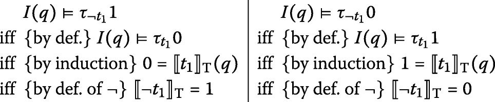
The correctness of Algorithm 1 essentially hinges on two lemmata, which we present next. The first one states that transformation τ faithfully characterizes sets of queries, whereas the second one states that transformation τ correctly encodes the simplified evaluation of the policy language. Note that using a simple structural induction, one can easily show that τ_t⊥=¬(τ_t1∨τ_t0) and π⊥(p)=¬(π1(p)∨π0(p)). Thus, in our proofs, we can focus on the cases d=1 and d=0.

Lemma 2

(a) For all $q \in Q_{\mathcal {A}}$, I(q)⊧τ_td iff d=⟦t⟧_T(q).

Proof

By structural induction on t. Let $q \in Q_{\mathcal {A}}$ be arbitrary.

• Base case: t ≡ (a,v). We prove correctness for each d ∈ {1, 0} separately (Recall that case d = ⊥ follows from d = 1 and d = 0).

  • Case d=1. Suppose I(q)⊧τ_(a,v)1. By definition, τ_(a,v)1=a_v. From this, it follows that I(q)⊧a_v which, by definition means that I(q)(a_v)=true and, thus, (a,v)∈q. By definition of ⟦·⟧_T we also have ⟦(a,v)⟧_T(q)=1.

  • Case d=0 follows identical reasoning using Table 3.

• Induction hypothesis: suppose that, for all d^′, $I(q) \models \tau _{t_{i}}{d^{\prime }} \text { iff} d^{\prime } = \llbracket t_{i} \rrbracket _{\mathrm {T}} (q)$ with i∈{1,2}. We need to consider all unary and binary operators and prove each equivalence for all d∈{1,0}. We provide details for negation ¬ and strong conjunction ; the proofs for all remaining operators are analogous and therefore omitted.

  • Suppose t≡¬t₁. We compute:

    

  • Suppose t≡t₁ t₂. We compute for d=1:

    

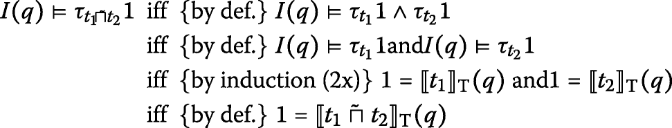
    Case d=0 follows the same reasoning, employing the encodings of Table 3.

□

Lemma 3

(b) For all $q \in Q_{\mathcal {A}}$, I(q)⊧π_d(p) iff d=⟦p⟧_B(q).

Proof

The proof of this lemma proceeds by induction on the structure of the policy. Since the proof bears many similarities to that of the previous lemma, we only highlight the interesting case, which is the case p≡(t,p₁). Assume, as our induction hypothesis, that for all d^′, $I(q) \models \pi _{d^{\prime }}(p_{1}) \text {iff} d^{\prime } = \llbracket p_{1} \rrbracket _{\mathrm {B}} (q)$.

We separately prove the statement for d∈{1,0}. We reason as follows:

□

Finally, we observe that the proposition R̄, defined as $\bigwedge \{ a_{v} \Rightarrow a_{v}^{\prime } \mid a_{v} \in {Vars}_{\mathcal {A}} \}$, indeed encodes the subset relation on $Q_{\mathcal {A}}$. We introduce an interpretation $I^{\prime } : Q_{\mathcal {A}} \to (Vars^{\prime } \rightarrow \mathbb {B})$, which is given by $I^{\prime }(q)\left (a_{v}^{\prime }\right) = true$ iff (a,v)∈q. We write η∪η^′⊧ R̄ iff R̄ holds under interpretation $\eta : Vars \rightarrow \mathbb {B}$ for variables from Vars and $\eta ^{\prime } : Vars^{\prime } \rightarrow \mathbb {B}$ for variables from Vars^′.

Lemma 4

For all $q,q^{\prime }\! \in \! Q_{\mathcal {A}}$, I(q)∪I^′(q^′)⊧ R̄ iff (q,q^′)∈→^∗.

Proof

First, observe that →^∗ is in fact equivalent to ⊆ on $Q_{\mathcal {A}}$.

• Implication from left to right. Suppose I(q)∪I^′(q^′)⊧ R̄. Then, $I(q) \cup I^{\prime }\left (q^{\prime }\right) \models \bigwedge \{ a_{v} \Rightarrow a_{v}^{\prime } \mid a_{v} \in {Vars}_{\mathcal {A}} \}$, and, therefore, for all $a_{v} \in {Vars}_{\mathcal {A}}$, we find that $I(q) \cup I^{\prime }\left (q^{\prime }\right) \models a_{v} \Rightarrow a_{v}^{\prime }$. But then if I(q)(a_v) holds, then so does $I^{\prime }\left (q^{\prime }\right)\left (a_{v}^{\prime }\right)$. By definition, this means (a,v)∈q implies (a,v)∈q^′ for all $(a,v) \in Q_{\mathcal {A}}$. But then q⊆q^′, or, equivalently (q,q^′)→^∗.

• Implication from right to left. Suppose (q,q^′)∈→^∗, or, equivalently, q⊆q^′. Pick some arbitrary $(a,v) \in Q_{\mathcal {A}}$, and assume (a,v)∈q. By definition, we then have I(q)(a_v) holds. Since q⊆q^′, also (a,v)∈q^′; but then also I^′(q)(a_v) holds. So we have I(q)(a_v) implies $I^{\prime }(q)\left (a_{v}^{\prime }\right)$. But then $I(q) \cup I^{\prime }\left (q^{\prime }\right) \models a_{v} \Rightarrow a_{v}^{\prime }$. Since we picked $(a,v) \in Q_{\mathcal {A}}$ arbitrary, we find that $I(q) \cup I^{\prime }\left (q^{\prime }\right) \models \bigwedge \left \{ a_{v} \Rightarrow a_{v}^{\prime } \mid a_{v} \in {Vars}_{\mathcal {A}} \right \}$.

□

The correctness of procedure COMPUTEEXTENDEDEVALUATION (Theorem 4) directly follows from the next proposition, where R= R̄ $\wedge S \wedge S \left [{Vars}_{\mathcal {A}} := {Vars}_{\mathcal {A}}^{\prime } \right ]$ and $S = \bigwedge \{\tau _{c}{1} \mid c \in C\}$:

Proposition B.1

For all d∈{1,0,⊥}, $q \in Q_{\mathcal {A} \mid C} \wedge d \in \llbracket p \rrbracket _{\mathrm {E}}(q)$ iff $I(q) \models (\pi _{d}(p) \wedge S) \vee \exists {Vars}_{\mathcal {A}}^{\prime }. \left (R \wedge (\pi _{d}(p))\left [{Vars}_{\mathcal {A}} := {Vars}_{\mathcal {A}}^{\prime }\right ] \right)$.

Proof

Follows from Lemmata 2, 3 and 4. □

References

Bahrak, B, Deshpande A, Whitaker M, Park J (2010) BRESAP: A Policy Reasoner for Processing Spectrum Access Policies Represented by Binary Decision Diagrams In: Proceedings of Symposium on New Frontiers in Dynamic Spectrum, 1–12.. IEEE.
Banzhaf, JF (1966) Multi-Member Electoral Districts. Do They Violate the “One Man, One Vote” Principle. Yale Law J 75(8):1309–1338.
Barrett, C, Conway CL, Deters M, Hadarean L, Jovanović D, King T, Reynolds A, Tinelli C (2011) CVC4 In: Proceedings of International Conference on Computer Aided Verification, LNCS, vol 6806, 171–177.. Springer, Berlin.
Bryant, RE (1992) Symbolic Boolean Manipulation with Ordered Binary-Decision Diagrams. ACM Comput Surv 24(3):293–318.
Crampton, J, Huth M (2010) An authorization framework resilient to policy evaluation failures, LNCS, vol 6345 In: Computer Security, 472–487.. Springer, Berlin.
Crampton, J, Morisset C (2012) PTaCL: A Language for Attribute-Based Access Control in Open Systems, LNCS, vol 7215 In: Principles of Security and Trust, 390–409.. Springer, Berlin.
Crampton, J, Morisset C, Zannone N (2015) On missing attributes in access control: Non-deterministic and probabilistic attribute retrieval In: Proceedings of Symposium on Access Control Models and Technologies, 99–109.. ACM, New York.
Crampton, J, Williams C (2016) On completeness in languages for attribute-based access control In: Proceedings of Symposium on Access Control Models and Technologies, 149–160.. ACM, New York.
Dolski, S, Huonder F, Oberholzer S (2007) HERAS-AF: XACML 2.0 Implementation. Tech. rep., University of Applied Sciences Rapperswil.
Fisler, K, Krishnamurthi S, Meyerovich L, Tschantz M (2005) Verification and change-impact analysis of access-control policies In: Proceedings of International Conference on Software Engineering, 196–205.. ACM, New York.
Hu, H, Ahn G, Kulkarni K (2013) Discovery and Resolution of Anomalies in Web Access Control Policies. IEEE Trans Dependable Secure Comput 10(6):341–354.
Kaluvuri, SP, Egner AI, den Hartog J, Zannone N (2015) SAFAX - an extensible authorization service for cloud environments. Front ICT 2.
Liu, A, Chen F, Hwang J, Xie T (2011) Designing fast and scalable XACML policy evaluation engines. IEEE Trans Comput 60(12):1802–1817.
Morisset, C, Willemse TAC, Zannone N (2018) Efficient extended ABAC evaluation In: Proceedings of Symposium on Access Control Models and Technologies, 149–160.. ACM, New York.
Morisset, C, Zannone N (2014) Reduction of access control decisions In: Proceedings of Symposium on Access Control Models and Technologies, 53–62.. ACM, New York.
OASIS (2005) eXtensible Access Control Markup Language (XACML) Version 2.0. OASIS Standard.
OASIS (2013) eXtensible Access Control Markup Language (XACML) Version 3.0. OASIS Standard.
Rudell, R (1993) Dynamic variable ordering for ordered binary decision diagrams In: Proceedings of International Conference on Computer Aided Design, 42–47.. IEEE, Los Alamitos.
Srinivasan, A, Ham T, Malik S, Brayton RK (1990) Algorithms for discrete function manipulation In: Proceedings of International Conference on Computer-Aided Design, 92–95.. IEEE.
Tschantz, M, Krishnamurthi S (2006) Towards reasonability properties for access-control policy languages In: Proceedings of Symposium on Access Control Models and Technologies, 160–169.. ACM, New York.
Turkmen, F, den Hartog J, Ranise S, Zannone N (2017) Formal analysis of XACML policies using SMT. Comput Secur 66:185–203.
Zhang, N, Ryan M, Guelev D (2005) Evaluating access control policies through model checking, LNCS, vol 3650 In: Information Security, 446–460.. Springer, Berlin.
Acknowledgments
Not applicable.
Funding
This work is partially funded by the ITEA3 project APPSTACLE (15017) and the ECSEL project SECREDAS (783119).
Availability of data and materials
Two access control policies used for the experiments are publicly available. The SAFAX policy cannot be disclosed due to a confidentiality agreement with project partners.
Author information
Authors and Affiliations
Contributions
All authors contributed equally and approved the final manuscript.
Corresponding author
Ethics declarations
Competing interests
The authors declare that they have no competing interests.
Publisher’s Note
Springer Nature remains neutral with regard to jurisdictional claims in published maps and institutional affiliations.
Rights and permissions
Open Access This article is distributed under the terms of the Creative Commons Attribution 4.0 International License(http://creativecommons.org/licenses/by/4.0/), which permits unrestricted use, distribution, and reproduction in any medium, provided you give appropriate credit to the original author(s) and the source, provide a link to the Creative Commons license, and indicate if changes were made.
About this article
Cite this article
Morisset, C., Willemse, T. & Zannone, N. A framework for the extended evaluation of ABAC policies. Cybersecur 2, 6 (2019). https://doi.org/10.1186/s42400-019-0024-0
Received:
Accepted:
Published:
DOI: https://doi.org/10.1186/s42400-019-0024-0