Efficient functional encryption for inner product with simulation-based security

Abstract

Functional encryption (FE) is a novel paradigm for encryption scheme which allows tremendous flexibility in accessing encrypted information. In FE, a user can learn specific function of encrypted messages by restricted functional key and reveal nothing else about the messages. Inner product encryption (IPE) is a special type of functional encryption where the decryption algorithm, given a ciphertext related to a vector x and a secret key related to a vector y, computes the inner product x·y. In this paper, we construct an efficient private-key functional encryption (FE) for inner product with simulation-based security, which is much stronger than indistinguishability-based security, under the External Decisional Linear assumption in the standard model. Compared with the existing schemes, our construction is faster in encryption and decryption, and the master secret key, secret keys and ciphertexts are shorter.

Introduction

Traditional public key encryption provides all-or-nothing access to data, either recovering the entire plaintext or revealing nothing from the ciphertext. Functional Encryption (FE) (Dan et al. 2011; O’Neill 2010) is a very useful tool for non-interactive computation on encrypted data. In FE, the owner of master secret key msk can create a secret key sk_f for a function f, which enables users to compute the value of f(x) by decrypting a ciphertext of x without revealing anything else about x. As cloud services are increasing rapidly, users’ demand for computation on encrypted data is also increasing because cloud servers are by no means trustful. FE is one solution to this problem, providing a paradigm where users can compute a function f on encrypted data using a secret key sk_f without revealing anything else about the encrypted data using data to the cloud server.

One of the principal interests in FE is what class of functions $\mathcal {F}$ can be supported and what kind of security can be achieved. It started from identity-based encryption (Boneh and Franklin 2001), followed by attributed-based encryption (Goyal et al. 2006), hidden vector encryption (Iovino and Persiano 2008; Caro et al. 2012) and predicate encryption (Katz et al. 2008; Shen et al. 2009). Amazingly, recent works realize computation of general polynomial-size circuits (Garg et al. 2016), although they require expensive assumptions like indistinguishability obfuscation, which are far from being practical. Motivated by this unreality, (Abdalla et al. 2015) introduced a new non-generic FE scheme specialized for computation of the evaluation of inner product values, which is efficient and constructed from standard assumptions. As (Abdalla et al. 2015) mentioned in their work, inner-product is a very useful tool for statistics because it can provide the weighted mean. In an inner product encryption (IPE) scheme, a ciphertext ct_x is related to a vector $\boldsymbol {x}\in \mathbb {Z}_{q}^{n}$ of length n and a secret key sk_y related to a vector $\boldsymbol {y}\in \mathbb {Z}_{q}^{n}$. Given the ciphertext and the secret key, the decryption algorithm computes the inner product $\boldsymbol {x}\cdot \boldsymbol {y}=\sum _{i=1}^{n} x_{i} y_{i}$. Note that FE for inner-product is different from inner-product encryption (IPE) in the context of predicate encryption. In the phase of encryption and secret key generation of the inner product encryption (predicate encryption), a secret key corresponds to a predicate vector $\boldsymbol {y}\in \mathbb {Z}_{q}^{n}$ and a ciphertext for a message m comes along with an attribute vector $\boldsymbol {x}\in \mathbb {Z}_{q}^{n}$, the decryption algorithm outputs m if x·y=0. By contrast, the result of the IPE scheme in this paper is the actual value of the inner product.

Private-key IPE has several practical applications (Kim et al. 2018; Zhao et al. 2018) as well, such as biometric authentication and nearest-neighbor search on encrypted data. Biometric-based authentication system is prevalent. It is well-known that biometrics are inherently noisy, authentication should be successful when the supplied biometric is close to a user’s credential stored in the system. It is achieved by computing the Hamming distance between them, which is the number of bits differing from each other. Private-key inner product encryption can be used to compute the Hamming distance between the bitstrings of two vectors. Another application of IPE is the nearest-neighbor search on encrypted data. Consider an encrypted database of files F. Given a file f, the problem of k-nearest neighbor search is to find the prior-k files in F that are the most similar to f. The common measure of file similarity is the Euclidean distance between the vector representations of files. Private-key IPE gives an efficient way of performing the nearest-neighbor search over an encrypted database. Readers could refer to (Kim et al. 2018; Zhao et al. 2018) for a detailed introduction to these applications of IPE.

Related works

The first construction of IPE was presented by Abdalla et al. (2015) who developed a selectively secure scheme under the indistinguishability-based security. Subsequently, (Agrawal et al. 2016) and (Abdalla et al. 2016) have designed adaptively secure IPE constructions where the messages x₀ and x₁ may be adaptively chosen in time, based on the previously collected information. However, these constructions are built with public key and do not support any forms of function privacy. Then, researchers explored the possibility of attaining function privacy in the context of IPE. Bishop et al. (2015) constructed a function-hiding IPE scheme in the private key domain under the well-studied Symmetric External Diffie-Hellman(SXDH) assumption, which satisfies an indistinguishability-based definition, and considered adaptive adversaries. Roughly speaking, an IPE scheme is function-hiding if the keys and ciphertexts reveal no additional information about both x and y beyond their inner product. However, their security model imposes a little unrealistic admissibility constraint on the adversary’s queries. All ciphertexts queries x₀,x₁ and all secret key queries y₀,y₁ are restrained by x₀·y₀=x₀·y₁=x₁·y₀=x₁·y₁.That makes the security of the scheme become weak. Datta et al. (2017) constructed a private-key function-hiding IPE scheme from the SXDH assumption that changed the restriction on adversaries’ queries is only x₀·y₀=x₁·y₁. In their construction, secret keys and ciphertexts of n-dimensional vectors consist of 4n+8 groups elements. This was further improved upon in a work by Tomida et al. (2016) who gave a construction of a private-key function hiding IPE from the DLIN assumption where the secret keys and ciphertexts consist of 2n+5 groups elements. Recently, (Kim et al. 2019) put forth a construction of function-hiding IPE scheme with less parameter sizes and run time complexity than in Bishop et al. (2015); Datta et al. (2017). The scheme is proved simulation-based secure in the generic model of bilinear maps.

There are also several research works about Inner product encryption (Agrawal et al. 2015; Caro et al. 2013; Goldwasser et al. 2014; Abdalla et al. 2017); (Datta et al. 2018), such as Multi-Input inner product encryption(MIPE) and predicate encryption for inner product (Okamoto and Takashima 2009; Attrapadung and Libert 2010; Lewko et al. 2010; Okamoto 2011; Park 2011; Okamoto and Takashima 2012a; Okamoto and Takashima 2012b; Kawai and Takashima 2013; Zhenlin and Wei 2015; Zhang et al. 2019). In Goldwasser et al. (2014) introduced the definition of Multi-Input functional encryption, the functions can be evaluated on encrypted information to take multiple inputs, with each input corresponding to a different ciphertext. Abdalla et al. (2017) constructed the first scheme of Multi-Input inner product encryption which achieves message privacy, and (Datta et al. 2018) proposed a new scheme which they call unbounded private-key Multi-Input inner product functional encryption. Their scheme achieved function-hiding privacy, meanwhile they enabled the encryption of ciphertexts, and the generation of secret keys for unbounded vectors. In Dufour-Sans and Pointcheval (2019), described an unbounded inner product encryption which supported identity access control with succinct keys. Their construction is proven selectively secure in the random-oracle model based on the standard DBDH assumption. Tomida and Takashima (2018) did the similar research, but their construction didn’t supported the function of identity access control. In Agrawal et al. (2020), resolved the question of simulation-based security for inner product encryption based on DDH, Paillier and LWE assumption. In 2008, the first predicate encryption for inner product was introduced by Katz et al. (2008), which allows evaluating predicates over $\mathbb {Z}_{N}$ using inner product, where N is a composite number. In Okamoto and Takashima (2009) proposed the first hierarchical predicate encryption for inner product predicate, which allows a user with functionality that can delegate more restrictive functionality to another user, but their schemes had low inefficiency. Attrapadung and Libert (2010); Lewko et al. (2010); Okamoto (2011) constructed their IPE schemes respectively, which improves the efficiency of the previous scheme. However, the security proof of all previous studies based on non-standard assumptions. In order to address this issue, (Park 2011) proposed the first IPE scheme under the standard assumptions (i.e., decisional bilinear Diffie-Hellman (DBDH) and decisional linear (DLIN) assumptions). Okamoto and Takashima (2012a) proposed the first IPE scheme that is fully secure and fully attribute-hiding, and then (Okamoto and Takashima 2012b) further proposed the first unbounded IPE scheme that is also fully secure and fully attribute-hiding in the standard model under DLIN assumption. Kawai and Takashima (2013) introduced a new concept, called IPE with ciphertext conversion, which takes into account the security of predicate hiding. Zhenlin and Wei (2015) introduced another notion, called multi-party cloud computation IPE with multiplicative homomorphic property, which enables IPE to support multi-party cloud computation. Zhang et al. (2019) proposed a new IPE scheme based on double encryption system, which is proven to be adaptive security under weak attribute hiding model.

A lot of the problems mentioned above will lead an IPE scheme impractical and takes us the following problem:

Can we optimize the length of the master secret key, ciphertexts and secret keys with the simulation-based security?

Our contribution

We construct a more efficient and flexible private-key IPE scheme with simulation-based security. To ensure correctness, our scheme requires that the computation of inner products is within a polynomial range (Datta et al. 2016), where discrete logarithm of g^x·y can be found in polynomial time.

Efficiency

Our scheme is constructed based on dual paring vector spaces (DPVS). Namely, a master secret key is orthonormal bases of DPVS, secret keys and ciphertexts are vectors of DPVS, both key generation algorithm and encryption algorithm involve scalar multiplications on cyclic groups, and a decryption algorithm involves paring operations on bilinear paring groups. Our scheme is superior to other schemes, in terms of both necessary storage and computational efficiency.

Assumption and flexibility

The schemes of Bishop et al. (2015); Datta et al. (2016) are secure under the symmetric external Diffie-Hellman (SXDH) assumption, while our scheme is based on decision linear (DLIN) assumption or its variant (XDLIN). SXDH holds in only Type-3 bilinear pairing groups, DLIN and XDLIN hold in any type of bilinear pairing groups, so DLIN and XDLIN are weaker assumptions than SXDH. For this reason, the schemes of Bishop et al. (2015)Datta et al. (2016) work in only Type-3 groups while we can use our scheme in any type of bilinear pairing groups.

Security

There are two notions of security for a FE scheme, indistinguishability-based security and simulation based security model. The former one requires that an adversary cannot distinguish between ciphertexts of any two messages m₀,m₁ with access to a secret key sk_f of function f such that f(m₀)=f(m₁). By contrast, the latter one requires that the view of the adversary can be simulated by a simulator, given only access to secret keys and functions evaluated on the corresponding messages. Note that simulation-based security has higher security strength than indistinguishability-based security such that there exists an indistinguishability-based secure FE scheme for a certain functionality which is not able to be proved secure under simulation-based security. Our scheme achieves simulation-based security, which is more secure than indistinguishability-based security.

Preliminary

Notation

For a set S, $x \stackrel {\mathsf {U}}{\leftarrow } S$ denotes that x is uniformly chosen from S. For a probability distribution $X,\ x \stackrel {\mathsf {R}}{\leftarrow } X$ denotes that x is chosen from X according to its distributions. For a prime $q,\ \mathbb {Z}_{q}$ denotes a set of integers {0,⋯,q−1}, and $\mathbb {Z}_{q}^{\times }$ denotes a set of integers {1,⋯,q−1},0 denotes a zero vector. For an n-dimensional vector x, x_i(1≤i≤n) denotes the i-th component of x. For vectors $\boldsymbol {x},\boldsymbol {y} \in \mathbb {Z}_{q}^{n},\ \boldsymbol {x} \cdot \boldsymbol {y} \$ denotes inner-product of x and y over $\mathbb {Z}_{q}$. For vector components, 0ⁿ denotes a line of n zeros, e.g., a:=(0,0,0,1)=(0³,1). Let $A=\{A_{n}\}_{n\in \mathbb {N}}$ and $B=\{B_{n}\}_{n\in \mathbb {N}}$ be distribution ensembles. We denote by A≈_cB that A and B are computationally indistinguishable. Let negl(λ) be a negligible function in λ. B^T denotes the transpose of matrix B. $GL(n,\mathbb {Z}_{q})$ denotes the general linear group of degree n over $\mathbb {Z}_{q}$.

Bilinear pairing groups

Bilinear pairing groups are defined by the tuple ($q,\mathbb {G}_{1},\mathbb {G}_{2},\mathbb {G}_{T},e$), where q is a prime, $\mathbb {G}_{1},\ \mathbb {G}_{2}$ and $\mathbb {G}_{T}$ are cyclic groups of order q, and e : $\mathbb {G}_{1} \times \mathbb {G}_{2} \rightarrow \mathbb {G}_{T}$ is a map that has the following properties:

• 1 Bilinearity: $\forall G_{1} \in \mathbb {G}_{1},\ \forall G_{2} \in \mathbb {G}_{2},\ \forall a,b \in \mathbb {Z}_{q},\ e(aG_{1},bG_{2})=e(G_{1},G_{2})^{ab}$.

• 2 Non-degeneracy: if $\forall G_{1} \in \mathbb {G}_{1},\ G_{1} \neq 0, \ e(G_{1},G_{2})=1$, then G₂=0.

There are three types of bilinear groups according to whether efficient isomorphisms exist or not between $\mathbb {G}_{1}$ and $\mathbb {G}_{2}$. In Type-1 bilinear groups, both the isomorphism ϕ: $\mathbb {G}_{2} \rightarrow \mathbb {G}_{1}$ and its inverse ϕ⁻¹: $\mathbb {G}_{1} \rightarrow \mathbb {G}_{2}$ can be computed efficiently, i.e., $\mathbb {G}_{1}$ = $\mathbb {G}_{2}$. In Type-2 bilinear groups, the isomorphism ϕ: $\mathbb {G}_{2} \rightarrow \mathbb {G}_{1}$ is computed efficiently but its inverse is not. Type-3 groups do not have efficient isomorphisms between $\mathbb {G}_{1}$ and $\mathbb {G}_{2}$. Type-1 groups are called symmetric bilinear pairing groups, and Type-2 and Type-3 are called asymmetric bilinear pairing groups. We use Type-3 groups to build our scheme in the paper. Let $\mathcal {G}_{\mathsf {abpg}}$ be an asymmetric bilinear pairing group generators that takes 1^λ and outputs a description of ($q,\mathbb {G}_{1},\mathbb {G}_{2},\mathbb {G}_{T},e$) and generators of groups $G_{1}\neq 0\in \mathbb {G}_{1},\ G_{2} \neq 0 \in \mathbb {G}_{2}$. We denote the tuple ($q,\mathbb {G}_{1},\mathbb {G}_{2},\mathbb {G}_{T},G_{1},G_{2},e$) by $\mathsf {param}_{\mathbb {G}}$.

Dual pairing vector space

Definition 1

(Lewko et al. 2010; Okamoto and Takashima 2009; Okamoto and Takashima 2015) (Dual Pairing Vector Spaces:DPVS): We briefly introduce the concept of DPVS. DPVS are defined by the tuple $(q,\mathbb {V},\mathbb {V}^{*},\mathbb {G}_{T},\mathbb {A},\mathbb {A}^{*},\widetilde {e})$, which is directly constructed from $\mathsf {param}_{\mathbb {G}} \stackrel {\mathsf {R}}{\leftarrow } \mathcal {G}_{\mathsf {abpg}} \left (1^{\lambda } \right).\ \mathbb {V}:=\mathbb {G}_{1}^{n}$ and $\mathbb {V}^{*}:=\mathbb {G}_{2}^{n}$ are n-dimensional vector spaces, $\mathbb {A}:=(\boldsymbol {a}_{1},\cdots,\boldsymbol {a}_{n})=\left [ \begin {array}{llll} G_{1} & 0 & \cdots & 0 \\ 0 & G_{1} & \cdots & 0 \\ \vdots & \vdots & \ddots & \vdots \\ 0 & 0 & \cdots & G_{1} \\ \end {array} \right ]$ and $\mathbb {A}^{*}:=(\boldsymbol {a}_{1}^{*},\cdots,\boldsymbol {a}_{n}^{*})=\left [ \begin {array}{llll} G_{2} & 0 & \cdots & 0 \\ 0 & G_{2} & \cdots & 0 \\ \vdots & \vdots & \ddots & \vdots \\ 0 & 0 & \cdots & G_{2} \\ \end {array} \right ]$ are canonical bases, where $\boldsymbol {a}_{i}:=\left (0^{i-1},G_{1},0^{n-i}\right), \boldsymbol {a}_{i}^{*}:=\left (0^{i-1},G_{2},0^{n-i}\right)$, and $\tilde {e}:\mathbb {V} \times \mathbb {V}^{*} \rightarrow \mathbb {G}_{T}$ is a pairing defined by $\tilde {e}(\boldsymbol {x},\boldsymbol {y}):= \prod _{i=1}^{n} e(X_{i},Y_{i}) \in \mathbb {G}_{T}$, where $\boldsymbol {x}:=(X_{1},\cdots,X_{n}) \in \mathbb {V},\ \boldsymbol {y}:=(Y_{1},\cdots,Y_{n}) \in \mathbb {V}^{*}$.

Let $(q,\mathbb {V},\mathbb {V}^{*},\mathbb {G}_{T}, \mathbb {A},\mathbb {A}^{*},\widetilde {e})$ be the output of algorithm $\mathcal {G}_{\mathsf {dpvs}} (1^{\lambda },n,\mathsf {param}_{\mathbb {G}})$, where $n \in \mathbb {N}$. Then we describe random dual orthonormal bases as follows:

We randomly select a new non-singular matrix X to do a linear transformation and achieve base change.

$$\begin{array}{*{20}l} \psi \stackrel{\mathsf{U}}{\leftarrow} \mathbb{Z}_{q}^{\times},\ \boldsymbol{X}&:=\left(\chi_{i,j}\right)_{1 \leq i,j \leq n} \stackrel{\mathsf{U}}{\leftarrow} GL\left(n,\mathbb{Z}_{q}\right),\ \left(\upsilon_{i,j}\right)_{1 \leq i,j \leq n}\\&:=\psi\left(\boldsymbol{X}^{T}\right)^{-1}, \end{array} $$

$$\begin{array}{*{20}l} \boldsymbol{b}_{i}&:= {\sum\nolimits}_{j=1}^{n} \chi_{i,j}\boldsymbol{a}_{j}= \left(\begin{array}{ccc} \boldsymbol{a}_{1} &\cdots &\boldsymbol{a}_{n} \end{array} \right) \left(\begin{array}{c} \chi_{i1} \\ \vdots \\ \chi_{in} \end{array} \right),\\ \boldsymbol{b}_{i}^{*}&:= {\sum\nolimits}_{j=1}^{n} \upsilon_{i,j} \boldsymbol{a}_{j}^{*}= \left(\begin{array}{ccc} \boldsymbol{a}_{1}^{*} &\cdots &\boldsymbol{a}_{n}^{*} \end{array} \right) \left(\begin{array}{c} \upsilon_{i1} \\ \vdots \\ \upsilon_{in} \end{array} \right)\\ &\qquad\text{for}\ i=1, \cdots, n, \end{array} $$

$$\begin{array}{*{20}l} \mathbb{B}&:=(\boldsymbol{b}_{1},\cdots,\boldsymbol{b}_{n}),\\ \mathbb{B}^{*}&:=(\boldsymbol{b}_{1}^{*},\cdots,\boldsymbol{b}_{n}^{*}),\\ g_{T}&:=e(G_{1},G_{2})^{\psi}. \end{array} $$

Let $\mathcal {G}_{\mathsf {ob}}$ be the random dual orthonormal basis generator that takes 1^λ and a dimension of bases n and outputs ($\mathsf {param}_{\mathbb {G}},\mathbb {B},\mathbb {B}^{*},g_{T}$), where $\mathbb {B},\mathbb {B}^{*},g_{T}$ are computed as above. We denote the combination($\mathsf {param}_{\mathbb {G}},g_{T}$) by $\mathsf {\mathsf {param}_{\mathbb {V}}}$. For a vector $\boldsymbol {x}=({x_{1},\cdots,x_{n}})^{T} \in \mathbb {Z}_{q}^{n}$ and a basis $\mathbb {B}:=(\boldsymbol {b}_{1},\cdots,\boldsymbol {b}_{n})$ we denote $\sum _{i=1}^{n} x_{i} \boldsymbol {b}_{i}=\\ \left (\begin {array}{ccc} x_{1} &\cdots & x_{n} \end {array} \right) \left (\begin {array}{c} \boldsymbol {b}_{1} \\ \vdots \\ \boldsymbol {b}_{n} \end {array} \right) \text {by} (\boldsymbol {x})_{\mathbb {B}}$. Then we have

$$\begin{array}{*{20}l} \tilde{e}\left(\left(\boldsymbol{x}\right)_{\mathbb{A}},(\boldsymbol{y})_{\mathbb{A}^{*}}\right)&=\prod_{i=1}^{n} e(x_{i}G_{1},y_{i}G_{2})\\&=e\left(G_{1},G_{2}\right)^{\sum_{i=1}^{n} x_{i}y_{i}}=e(G_{1},G_{2})^{\boldsymbol{x}\cdot\boldsymbol{y}}, \end{array} $$

so

$$\begin{array}{*{20}l} \tilde{e}\left(\left(\boldsymbol{x}\right)_{\mathbb{B}},\left(\boldsymbol{y}\right)_{\mathbb{B}^{*}}\right)&=\tilde{e}\left(\left(\boldsymbol{X}\boldsymbol{x}\right)_{\mathbb{A}},\left(\psi\left(\boldsymbol{X}^{T}\right)^{-1} \boldsymbol{y}\right)_{{\mathbb{A}^{*}}}\right)\\ &=e\left(G_{1},G_{2}\right)^{\psi \boldsymbol{X}\boldsymbol{x} \cdot \left(\boldsymbol{X}^{T}\right)^{-1} \boldsymbol{y}}=g_{T}^{\boldsymbol{x} \cdot \boldsymbol{y}}. \end{array} $$

External decision linear assumption

Definition 2

(Abe et al. 2016) We choose an arbitrary number x∈{1,2}. The XDLIN problem is to guess a bit b∈{0,1}, given P_b, where

$$ \mathsf{param}_{\mathbb{G}} \stackrel{R}{\leftarrow} \mathcal{G}_{\mathsf{abpg}} \left(1^{\lambda}\right),\ \xi,\kappa,\delta,\sigma,\rho \stackrel{U}{\leftarrow}\mathbb{Z}_{q}, $$

$$Y_{0}=(\delta + \sigma)G_{x},\ Y_{1}=(\delta + \sigma + \rho)G_{x}, $$

$$\begin{array}{*{20}l} P_{b}&=\left(\mathsf{param}_{\mathbb{G}},\xi G_{1},\kappa G_{1},\delta \xi G_{1},\right.\\ &\left.\quad\sigma \kappa G_{1}, \xi G_{2},\kappa G_{2},\delta \xi G_{2},\sigma \kappa G_{2},Y_{b}\right). \end{array} $$

For any probabilistic polynomial time (PPT) adversary $\mathcal {A}$, if its advantage (defined as below) in solving XDLIN problem is negligible in λ, we say that the XDLIN assumption holds. Namely,

$$\begin{array}{*{20}l} \mathsf{Adv}{{~}_{\mathcal{A}}}^{\mathsf{XDLIN}}(\lambda)&=\mathsf{Pr}\left[\mathcal{A}(1^{\lambda},P_{0}) \rightarrow 1\right]\\&-\mathsf{Pr}\left[\mathcal{A}(1^{\lambda},P_{1}) \rightarrow 1\right] \leq negl(\lambda). \end{array} $$

Private-key inner product encryption

A private-key IPE scheme is composed of the following four PPT algorithms.

• IPE.Setup(1^λ,n)→(msk,pp): The setup algorithm takes as input the security parameters 1^λ and vector length n. Then it outputs a master secret key msk and public parameters pp.

• IPE.Encrypt(msk,pp,x)→ct_x: The encryption algorithm takes as input the master secret key msk, the public parameters pp, and a vector $\boldsymbol {x} \in \mathbb {Z}_{q}^{n}$. Then it outputs a ciphertext ct_x.

• IPE.KeyGen(msk,pp,y)→sk_y: The key generation algorithm takes as input the master secret key msk, the public parameters pp, and a vector $\boldsymbol {y} \in \mathbb {Z}_{q}^{n}$. Then it outputs a secret key sk_y.

• $\mathsf {IPE.Decryption}\left (pp,ct_{\boldsymbol {x}},sk_{\boldsymbol {y}}\right)\rightarrow m \in \mathbb {Z}_{q}$ or ⊥: The decryption algorithm takes as input the public parameters pp, a ciphertext ct_x and a secret key sk_y. Then it outputs either a value $m= \boldsymbol {x} \cdot \boldsymbol {y} \in \mathbb {Z}_{q}$ or a dedicated symbol ⊥.

Simulation-based security

The simulation-based security (Caro et al. 2013; O’Neill 2010) in the Fig. 1 tries to capture the intuition that anything the adversary can compute from a ciphertext and the secret keys can be computed from the secret keys and the values of the corresponding functions on the underlying message. For an IPE scheme, if there exists a PPT adversary $\mathcal {A}=(\mathcal {A}_{1},\mathcal {A}_{2})$ and a PPT simulator $\mathcal {S}$, we define two experiments $\mathbf {REAL}_{\mathcal {A}}\left (1^{\lambda }\right),\ \mathbf {IDEAL}_{\mathcal {A},\mathcal {S}}\left (1^{\lambda }\right)$ in the box, let q₁ be the number of challenge messages output by $\mathcal {A}_{1}$ and q₂ be the number of secret key queries in the first stage. The oracle $\mathcal {O}$ and $\mathcal {O}^{\prime }$ are defined as follows:

• 1 The oracle $\mathcal {O}(msk,\cdot)=\mathsf {IPE.KeyGen}(msk,\cdot,\cdot)$.

  Fig. 1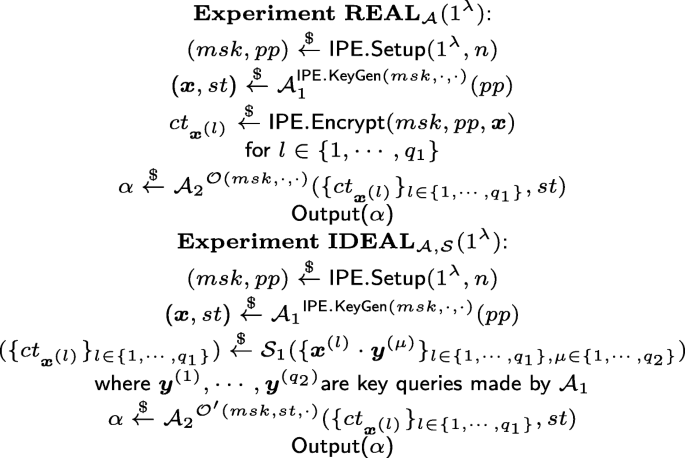

  

  Simulation-based security

• 2 The oracle $\mathcal {O}^{\prime }(msk,st,\cdot)$ is the second stage of the simulator, namely algorithm $\mathcal {S}^{\left \{\boldsymbol {x}^{(l)}\cdot \boldsymbol {y}^{(\mu)}\right \}}(msk,st,\cdot)$, for l∈{1,⋯,q₁}, μ∈{1,⋯,q₂}, where x^(l) and y^(μ) are inputs of the l-th ciphertext query and the μ-th secret key query by $\mathcal {A}_{1}$, respectively. Note that the simulator algorithm $\mathcal {S}$ is stateful so that after each invocation, it updates the state st which is carried over to its next invocation.

An IPE scheme is simulation-based secure if there exists a PPT simulator $\mathcal {S}$ such that, for all PPT adversaries $\mathcal {A}$, the outputs of the following two experiments are computationally indistinguishable:

$$\mathbf{REAL}_{\mathcal{A}}\left(1^{\lambda}\right) \approx_{c} \mathbf{IDEAL}_{\mathcal{A},\mathcal{S}}\left(1^{\lambda}\right).$$

Preliminary problems of security proof

In this section, we will introduce six lemmas and their security proofs. we firstly consider the following problems and use them to prove the security of our scheme.

Definition 3

Problem1 is to guess b∈{0,1}, given $\left (\mathsf {param}_{\mathbb {V}},\mathbb {B},\widehat {\mathbb {B}}^{*},\boldsymbol {y}_{b},\kappa G_{1},\xi G_{2}\right)$, where

$$ \mathsf{param}_{\mathbb{G}} \stackrel{\mathsf{R}}{\leftarrow} \mathcal{G}_{\mathsf{abpg}}\left(1^{\lambda}\right), $$

$$\begin{array}{*{20}l} \boldsymbol{X}&:=\left(\chi_{i,j}\right)_{1 \leq i,j \leq 3} \stackrel{\mathsf{U}}{\leftarrow} GL\left(3,\mathbb{Z}_{q}\right),\ \left(\upsilon_{i,j}\right)_{1 \leq i,j \leq 3}\\&:=\left(\boldsymbol{X}^{T}\right)^{-1}, \end{array} $$

$$\begin{array}{*{20}l} \kappa,\xi \stackrel{\mathsf{U}}{\leftarrow} \mathbb{Z}_{q}^{\times},\ \boldsymbol{b}_{i}&:= \kappa {\sum\nolimits}_{j=1}^{3} \chi_{i,j}\boldsymbol{a}_{j},\ \boldsymbol{b}_{i}^{*}\\&:= \xi {\sum\nolimits}_{j=1}^{3} \upsilon_{i,j} \boldsymbol{a}_{j}^{*}\ \text{for}\ i=1, 2, 3, \end{array} $$

$$\mathbb{B}:=(\boldsymbol{b}_{1},\boldsymbol{b}_{2},\boldsymbol{b}_{3}),\ {\widehat{\mathbb{B}}^{*}}:=\left(\boldsymbol{b}_{1}^{*},\boldsymbol{b}_{3}^{*}\right), $$

$$g_{T}:=e\left(G_{1},G_{2}\right)^{\kappa \xi}, $$

$$\begin{array}{*{20}l} \delta,\sigma \stackrel{\mathsf{U}}{\leftarrow} \mathbb{Z}_{q},\ \rho \stackrel{\mathsf{U}}{\leftarrow} \mathbb{Z}_{q}^{\times},\ \boldsymbol{y}_{0}&=(\delta,0,\sigma)_{\mathbb{B}} \text{and}\\ \boldsymbol{y}_{1}&=(\delta,\rho,\sigma)_{\mathbb{B}}. \end{array} $$

Definition 4

Problem1 ^′ is to guess b∈{0,1}, given $(\mathsf {param}_{\mathbb {V}},\mathbb {B}^{*},\widehat {\mathbb {B}},\boldsymbol {y}_{b}^{*},\kappa G_{1},\xi G_{2})$, where

$$\mathsf{param}_{\mathbb{G}} \stackrel{\mathsf{R}}{\leftarrow} \mathcal{G}_{\mathsf{abpg}}\left(1^{\lambda}\right), $$

$$\begin{array}{*{20}l} \boldsymbol{X}&:=(\chi_{i,j})_{1 \leq i,j \leq 3} \stackrel{\mathsf{U}}{\leftarrow} GL\left(3,\mathbb{Z}_{q}\right),\ (\upsilon_{i,j})_{1 \leq i,j \leq 3}\\&:=\left(\boldsymbol{X}^{T}\right)^{-1}, \end{array} $$

$$\begin{array}{*{20}l} \kappa,\xi \stackrel{\mathsf{U}}{\leftarrow} \mathbb{Z}_{q}^{\times},\ \boldsymbol{b}_{i}&:= \kappa {\sum\nolimits}_{j=1}^{3} \chi_{i,j}\boldsymbol{a}_{j},\ \boldsymbol{b}_{i}^{*}\\&:= \xi {\sum\nolimits}_{j=1}^{3} \upsilon_{i,j} \boldsymbol{a}_{j}^{*}\ \text{for}\ i=1, 2, 3, \end{array} $$

$$\mathbb{B}^{*}:=(\boldsymbol{b}_{1}^{*},\boldsymbol{b}_{2}^{*},\boldsymbol{b}_{3}^{*}),\widehat{\mathbb{B}}:=(\boldsymbol{b}_{1},\boldsymbol{b}_{3}), $$

$$g_{T}:=e\left(G_{1},G_{2}\right)^{\kappa \xi}, $$

$$\begin{array}{*{20}l} \delta,\sigma \stackrel{\mathsf{U}}{\leftarrow} \mathbb{Z}_{q},\ \rho \stackrel{\mathsf{U}}{\leftarrow} \mathbb{Z}_{q}^{\times},\ \boldsymbol{y}_{0}^{*}&=(\delta,0,\sigma)_{\mathbb{B}^{*}} \text{and} \boldsymbol{y}_{1}^{*}\\ &=(\delta,\rho,\sigma)_{\mathbb{B}^{*}}. \end{array} $$

Definition 5

Problem2 is to guess a bit b∈{0,1}, given $\left (\mathsf {param}_{\mathbb {V}},\widehat {\mathbb {B}},\widehat {\mathbb {B}}^{*},\boldsymbol {g}_{b}\right)$, where

$$(\mathbb{B},\mathbb{B}^{*},\mathsf{param}_{\mathbb{V}}) \stackrel{\mathsf{U}}{\leftarrow} \mathcal{G}_{\mathsf{ob}}\left(1^{\lambda},n+5\right), $$

$$\widehat{\mathbb{B}}=\left\{\boldsymbol{b}_{1},\cdots,\boldsymbol{b}_{n},\boldsymbol{b}_{n+1},\boldsymbol{b}_{n+3}\right\}, $$

$$\widehat{\mathbb{B}}^{*}=\left\{\boldsymbol{b}_{1}^{*},\cdots,\boldsymbol{b}_{n}^{*},\boldsymbol{b}_{n+2}^{*},\boldsymbol{b}_{n+4}^{*}\right\}, $$

$$\alpha,\eta \stackrel{\mathsf{U}}{\leftarrow} \mathbb{Z}_{q},\ \gamma^{\prime} \stackrel{\mathsf{U}}{\leftarrow} \mathbb{Z}_{q}^{\times}, $$

$$\boldsymbol{g}_{0}=\left(0^{n},\alpha,0,\eta,0,0\right)_{\mathbb{B}} \text{and} \boldsymbol{g}_{1}=\left(0^{n},\alpha,0,\eta,0,{\gamma}^{\prime}\right)_{\mathbb{B}}. $$

Definition 6

Problem3 is to guess a bit b∈{0,1}, given $\left (\mathsf {param}_{\mathbb {V}},\widehat {\mathbb {B}},\widehat {\mathbb {B}}^{*},\boldsymbol {g}_{b}\right)$, where

$$(\mathbb{B},\mathbb{B}^{*},\mathsf{param}_{\mathbb{V}})\stackrel{\mathsf{R}}{\leftarrow} \mathcal{G}_{\mathsf{ob}}\left(1^{\lambda},n+5\right), $$

$$\widehat{\mathbb{B}}=\left\{\boldsymbol{b}_{1},\cdots,\boldsymbol{b}_{n},\boldsymbol{b}_{n+1},\boldsymbol{b}_{n+5}\right\}, $$

$$\widehat{\mathbb{B}}^{*}=\left\{\boldsymbol{b}_{1}^{*},\cdots,\boldsymbol{b}_{n}^{*},\boldsymbol{b}_{n+2}^{*},\boldsymbol{b}_{n+4}^{*}\right\}, $$

$$\alpha,\eta \stackrel{\mathsf{U}}{\leftarrow} \mathbb{Z}_{q},\ \gamma^{\prime} \stackrel{\mathsf{U}}{\leftarrow} \mathbb{Z}_{q}^{\times}, $$

$$\boldsymbol{g}_{0}=\left(0^{n},\alpha,0,\eta,0,{\gamma}^{\prime}\right)\text{and} \boldsymbol{g}_{1}=\left(0^{n},\alpha,0,0,0, {\gamma}^{\prime}\right)_{\mathbb{B}}. $$

Definition 7

Problem4 is to guess a bit b∈{0,1}, given $\left (\mathsf {param}_{\mathbb {V}},\widehat {\mathbb {B}},\widehat {\mathbb {B}}^{*},\boldsymbol {g}_{b}^{*}\right)$, where

$$ (\mathbb{B},\mathbb{B}^{*},\mathsf{param}_{\mathbb{V}}) \stackrel{\mathsf{R}}{\leftarrow} \mathcal{G}_{\mathsf{ob}}\left(1^{\lambda},n+5\right), $$

$$\widehat{\mathbb{B}}={\left\{\boldsymbol{b}_{1},\cdots,\boldsymbol{b}_{n},\boldsymbol{b}_{n+1},\boldsymbol{b}_{n+5}\right\}}, $$

$$\widehat{\mathbb{B}}^{*}={\left\{\boldsymbol{b}_{1}^{*},\cdots,\boldsymbol{b}_{n}^{*},\boldsymbol{b}_{n+2}^{*},\boldsymbol{b}_{n+4}^{*}\right\}}, $$

$$\beta,\theta \stackrel{\mathsf{U}}{\leftarrow} \mathbb{Z}_{q},\ \tau^{\prime} \stackrel{\mathsf{U}}{\leftarrow} \mathbb{Z}_{q}^{\times}, $$

$$\boldsymbol{g}_{0}^{*}=\left(0^{n},0,\beta,0,\theta,0\right)_{\mathbb{B}^{*}}\text{and} \boldsymbol{g}_{1}^{*}=\left(0^{n},0,\beta,{\tau}^{\prime},\theta,0\right)_{\mathbb{B}^{*}}. $$

Definition 8

Problem5 is to guess a bit b∈{0,1}, given $\left (\mathsf {param}_{\mathbb {V}},\widehat {\mathbb {B}},\widehat {\mathbb {B}}^{*},\boldsymbol {g}_{b}^{*}\right)$, where

$$(\mathbb{B},\mathbb{B}^{*},\mathsf{param}_{\mathbb{V}})\stackrel{\mathsf{R}}{\leftarrow} \mathcal{G}_{\mathsf{ob}}\left(1^{\lambda},n+5\right), $$

$$\widehat{\mathbb{B}}:=\left(\boldsymbol{b}_{1},\cdots,\boldsymbol{b}_{n},\boldsymbol{b}_{n+1},\boldsymbol{b}_{n+5}\right), $$

$$\widehat{\mathbb{B}}^{*}:={\left\{\boldsymbol{b}_{1}^{*},\cdots,\boldsymbol{b}_{n}^{*},\boldsymbol{b}_{n+2}^{*},\boldsymbol{b}_{n+3}^{*}\right\}}, $$

$$\beta,\theta \stackrel{\mathsf{U}}{\leftarrow} \mathbb{Z}_{q},\ \tau^{\prime} \stackrel{\mathsf{U}}{\leftarrow} \mathbb{Z}_{q}^{\times}, $$

$$\boldsymbol{g}_{0}^{*}=\left(0^{n},0,\beta,{\tau}^{\prime},\theta,0\right)_{\mathbb{B}^{*}}\text{and} \boldsymbol{g}_{1}^{*}=\left(0^{n},0,\beta,{\tau}^{\prime},0,0\right)_{\mathbb{B}^{*}}. $$

For a PPT algorithm $\mathcal {A}$, the advantage of $\mathcal {A}$ against Problem n (n=1,1^′,2,3,4,5) is defined as

$$\begin{array}{*{20}l} \mathsf{Adv}_{\mathcal{A}}^{\mathsf{Pn}}(\lambda) &:=\left|\mathsf{Pr}\left[\mathcal{A}(1^{\lambda},P_{0})\rightarrow 1\right]\right.\\&\left.-\mathsf{Pr}\left[\mathcal{A}(1^{\lambda},P_{1})\rightarrow 1\right] \right|, \end{array} $$

where P_b is an instance of Problem n defined above. Then following six lemmas hold.

Lemma 1

For all PPT adversary $\mathcal {B}$ for Problem1, there exists a PPT adversary $\mathcal {A}$ such that $\mathsf {Adv}_{\mathcal {B}}^{\mathsf {P1}}(\lambda) \leq \mathsf {Adv}_{\mathcal {A}}^{\mathsf {XDLIN}}(\lambda)+5/q$.

Proof

We construct a PPT adversary $\mathcal {A}$ for the XDLIN problem from any PPT adversary $\mathcal {B}$ for Problem1. $\mathcal {A}$ is given an instance of XDLIN problem and sets

$$g_{T}:=e(\kappa G_{1},\xi G_{2}),\ \mathsf{param}_{\mathsf{P1}}:=({\mathsf{param}}_{\mathbb{G}},g_{T}), $$

$$\begin{array}{*{20}l} \boldsymbol{u}_{1}&:=(\xi,0,1)_{\mathbb{A}}=(\xi G_{1},0,G_{1}),\\ \boldsymbol{u}_{2}&:=(0,0,1)_{\mathbb{A}}=(0,0,G_{1}),\\ \boldsymbol{u}_{3}&:=(0,\kappa,1)_{\mathbb{A}}=(0,\kappa G_{1},G_{1}), \end{array} $$

$$\begin{array}{*{20}l} \boldsymbol{u}_{1}^{*}&:=(\kappa,0,0)_{\mathbb{A}^{*}}=(\kappa G_{2},0,0),\\ \boldsymbol{u}_{2}^{*}&:=(-\kappa,-\xi,\kappa \xi)_{\mathbb{A}^{*}}=(-\kappa G_{2},-\xi G_{2},\kappa \xi G_{2}),\\ \boldsymbol{u}_{3}^{*}&:=(0,\xi,0)_{\mathbb{A}^{*}}=(0,\xi G_2,0), \end{array} $$

$$\boldsymbol{w}_b:=(\delta \xi G_1,\sigma \kappa G_1,Y_b). $$

$\mathcal {A}$ can compute $\boldsymbol {u}_1,\boldsymbol {u}_2,\boldsymbol {u}_3,\boldsymbol {u}_{1}^{*},\boldsymbol {u}_{3}^{*}$. Then it generates a random linear transformation W on $\mathbb {G}^{3}$ to get a new group of bases and sets

$$\begin{array}{*{20}l}\boldsymbol{b}_i&:=W(\boldsymbol{u}_i) \text{for} \ {i} = 1,2,3\\ \boldsymbol{b}_{i}^{*}&:=(W^{-1})^{T}(\boldsymbol{u}_{i}^{*}) \text{for}\ \ {i}= 1,3, \end{array} $$

$$\mathbb{B}:=(\boldsymbol{b}_1,\boldsymbol{b}_2,\boldsymbol{b}_3), \widehat{\mathbb{B}}^{*}:=(\boldsymbol{b}_{1}^{*},\boldsymbol{b}_{3}^{*}), \boldsymbol{y}_b:=W(\boldsymbol{w}_b). $$

Then $\mathcal {A}$ gives $\left (\mathsf {param}_{P1},\mathbb {B},\widehat {\mathbb {B}}^{*},\boldsymbol {y}_b,\kappa G_1,\xi G_{2}\right)$ to $\mathcal {B}$, and outputs b^′ if $\mathcal {B}$ outputs b^′,

If b=0 and Y_b=Y₀=(δ+σ)G₁, then $\boldsymbol {w}_0=\left (\delta \xi G_1,\sigma \kappa G_1,\left (\delta +\sigma \right)G_{1}\right)=\left (\delta \xi,\sigma \kappa,\left (\delta +\sigma \right)\right)_{\mathbb {A}}=\delta \boldsymbol {u}_1+\sigma \boldsymbol {u}_{2}$ and $\boldsymbol {y}_0=W(\boldsymbol {w}_0)=W(\delta \boldsymbol {u}_1+\sigma \boldsymbol {u}_2)=(\delta,0,\sigma)_{\mathbb {B}}$, when κ,ξ≠0, with probability 2/q.

If b=1 and Y_b=Y₁=(δ+ρ+σ)G₁, then $\boldsymbol {w}_1=\left (\delta \xi G_1,\sigma \kappa G_1,\left (\delta +\rho +\sigma \right)G_{1}\right)=\left (\delta \xi,\sigma \kappa,\left (\delta +\sigma +\rho \right)\right)_{\mathbb {A}}=\delta \boldsymbol {u}_1+\rho \boldsymbol {u}_2+\sigma \boldsymbol {u}_{3}$ and $\boldsymbol {y}_1=W(\boldsymbol {w}_1)=W(\delta \boldsymbol {u}_1+\rho \boldsymbol {u}_2+\sigma \boldsymbol {u}_3)=(\delta,\rho,\sigma)_{\mathbb {B}}$, when κ,ξ,ρ≠0, except with probability 3/q.

It is the same as an instance of Problem1. If $\mathcal {B}$ succeeds in solving Problem1, so does $\mathcal {A}$ in solving XDLIN porblem. □

Lemma 2

For all PPT adversary $\mathcal {B}$ for Problem1 ^′, there exists a PPT adversary $\mathcal {A}$ such that $\mathsf {Adv}_{\mathcal {B}}^{\mathsf {P1}^{\prime }}(\lambda) \leq \mathsf {Adv}_{\mathcal {A}}^{\mathsf {XDLIN}}(\lambda)+5/q$.

Proof

The proof follows in the same condition as Lemma 1. □

Lemma 3

For all PPT adversary $\mathcal {B}$ for Problem2, there exists a PPT adversary $\mathcal {A}$ such that $\mathsf {Adv}_{\mathcal {B}}^{\mathsf {P2}}\left (\lambda \right) \leq \mathsf {Adv}_{\mathcal {A}}^{\mathsf {P1}}(\lambda)$.

Proof

We construct a PPT adversary $\mathcal {A}$ for Problem1 from any PPT adversary $\mathcal {B}$ for Problem2. $\mathcal {A}$ is given an instance of Problem1$\left (\mathsf {param}_{\mathsf {P1}},\mathbb {B},\widehat {\mathbb {B}}^{*},\boldsymbol {y}_b,\kappa G_1,\xi G_{2}\right)$. Then $\mathcal {A}$ generates a random linear transformation W on $\mathbb {G}^{n+5}$, and sets

$$\begin{array}{*{20}l} \mathsf{param}_{\mathbb{V}}:&=\mathsf{param}_{\mathsf{P1}}\\ \boldsymbol{d}_i:&=W\left(0^{i+2},\kappa G_1,0^{n+2-i}\right) \text{for}\ i=1,\cdots,n \\ \boldsymbol{d}_{n+1}:&=W\left(\boldsymbol{b}_1,0^{n+2}\right), \boldsymbol{d}_{n+2}:=W\left(0^{n+2},\kappa G_1,0^{2}\right), \\ \boldsymbol{d}_{n+3}:&=W\left(\boldsymbol{b}_3,0^{n+2}\right), \boldsymbol{d}_{n+4}:=W\left(0^{n+4},\kappa G_{1}\right),\\ \boldsymbol{d}_{n+5}:&=W\left(\boldsymbol{b}_2,0^{n+2}\right), \\ \boldsymbol{d}_{i}^{*}:&=\left(\left(W\right)^{-1}\right)^{T}\left(0^{i+2},\xi G_2,0^{n+2-i}\right)\\ &\qquad\text{for}\ i=1,\cdots,n \\ \boldsymbol{d}_{n+1}^{*}:&=\left(\left(W\right)^{-1}\right)^{T}\left(\boldsymbol{b}_{1}^{*},0^{n+2}\right),\\ \boldsymbol{d}_{n+2}^{*}&:=W\left(0^{n+2},\xi G_2,0^{2}\right), \\ \boldsymbol{d}_{n+3}^{*}:&=\left(\left(W\right)^{-1}\right)^{T}\left(\boldsymbol{b}_{3}^{*},0^{n+2}\right),\\ \boldsymbol{d}_{n+4}^{*}&:=\left(\left(W\right)^{-1}\right)^{T}\left(0^{n+4},\xi G_{2}\right),\\ \boldsymbol{d}_{n+5}^{*}:&=W\left(\boldsymbol{b}_{2}^{*},0^{n+2}\right), \\ \boldsymbol{h}_b&=W\left(\boldsymbol{y}_b,0^{n+2}\right) \\ \mathbb{D}:&=\left(\boldsymbol{d}_1,\cdots,\boldsymbol{d}_{n+5}\right),\ \mathbb{D}^{*}:=\left(\boldsymbol{d}_{1}^{*},\cdots,\boldsymbol{d}_{n+5}^{*}\right) \end{array} $$

We can see that ($\mathbb {D},\mathbb {D}^{*}$) are dual orthonormal bases. $\mathcal {A}$ does not have $\boldsymbol {b}_{2}^{*}$ but it can compute

$$\begin{array}{*{20}l} \widehat{\mathbb{D}}&:=\left(\boldsymbol{d}_{1},\cdots,\boldsymbol{d}_{n},\boldsymbol{d}_{n+1},\boldsymbol{d}_{n+3}\right),\\ \widehat{\mathbb{D}}^{*}&:=\left(\boldsymbol{d}_{1}^{*},\cdots,\boldsymbol{d}_{n}^{*},\boldsymbol{d}_{n+2}^{*},\boldsymbol{d}_{n+4}^{*}\right) \end{array} $$

Then $\mathcal {A}$ gives$\left (\mathsf {param}_{\mathbb {V}},\widehat {\mathbb {D}},\widehat {\mathbb {D}}^{*},\boldsymbol {h}_{b}\right)$ to $\mathcal {B}$, and outputs b^′ if $\mathcal {B}$ outputs b^′. We can see that $\boldsymbol {h}_0:=\left (0^{n},\alpha,0,\eta,0,0\right)_{\mathbb {D}},\ \boldsymbol {h}_1:=(0^{n},\alpha,0,\eta,0,\gamma ^{\prime })_{\mathbb {D}}$, where α:=δ,η:=σ and γ^′:=ρ. It is the same as an instance of Problem2. If $\mathcal {B}$ succeeds in solving Problem2, so does $\mathcal {A}$ in solving XDLIN problem. □

Lemma 4

For all PPT adversary $\mathcal {B}$ for Problem3, there exists a PPT adversary $\mathcal {A}$ such that $\mathsf {Adv}_{\mathcal {B}}^{\mathsf {P3}}(\lambda) \leq \mathsf {Adv}_{\mathcal {A}}^{\mathsf {P1}}(\lambda)$.

Proof

We can construct a PPT adversary $\mathcal {A}$ for Problem1 from any PPT adversary $\mathcal {B}$ for Problem3. $\mathcal {A}$ is given an instance of Problem1, ($\mathsf {param}_{\mathsf {P1}},\mathbb {B},\widehat {\mathbb {B}}^{*},\boldsymbol {y}_b,\kappa G_1,\xi G_{2}$). Then $\mathcal {A}$ generates a random linear transformation W on $\mathbb {G}^{n+5}$, and sets

$$\begin{array}{*{20}l} \mathsf{param}_{\mathbb{V}}:&=\mathsf{param}_{\mathsf{P1}},\\ \boldsymbol{d}_i:&=W\left(0^{i+2},\kappa G_1,0^{n+2-i}\right) \text{for}\ i=1,\cdots,n \\ \boldsymbol{d}_{n+1}:&=W\left(\boldsymbol{b}_1,0^{n+2}\right), \boldsymbol{d}_{n+2}:=W\left(0^{n+2},\kappa G_1,0^{2}\right),\\ \boldsymbol{d}_{n+3}:&=W\left(\boldsymbol{b}_2,0^{n+2}\right), \boldsymbol{d}_{n+4}:=W\left(0^{n+4},\kappa G_{1}\right),\\ \boldsymbol{d}_{n+5}:&=W\left(\boldsymbol{b}_3,0^{n+2}\right),\\ \boldsymbol{d}_{i}^{*}:&=W\left(0^{i+2},\xi G_2,0^{n+2-i}\right) \text{for}\ i=1,\cdots,n \\ \boldsymbol{d}_{n+1}^{*}:&=\left(\left(W\right)^{-1}\right)^{T}\left(\boldsymbol{b}_{1}^{*},0^{n+2}\right),\\ \boldsymbol{d}_{n+2}^{*}&:=\left(\left(W\right)^{-1}\right)^{T}\left(0^{n+2},\xi G_2,0^{2}\right),\\ \boldsymbol{d}_{n+3}^{*}:&=\left(\left(W\right)^{-1}\right)^{T}\left(\boldsymbol{b}_{2}^{*},0^{n+2}\right),\\ \boldsymbol{d}_{n+4}^{*}&:=\left(\left(W\right)^{-1}\right)^{T}\left(0^{n+4},\xi G_{2}\right),\\ \boldsymbol{d}_{n+5}^{*}:&=\left(\left(W\right)^{-1}\right)^{T}\left(\boldsymbol{b}_{3}^{*},0^{n+2}\right),\\ \boldsymbol{h}_b&=W\left(\boldsymbol{y}_b,0^{n+2}\right)\\ \mathbb{D}:&=\left(\boldsymbol{d}_1,\cdots,\boldsymbol{d}_{n+5}\right),\ \mathbb{D}^{*}:=\left(\boldsymbol{d}_{1}^{*},\cdots,\boldsymbol{d}_{n+5}^{*}\right) \end{array} $$

We can see that ($\mathbb {D},\mathbb {D}^{*}$) are dual orthonormal bases. $\mathcal {A}$ does not have $\boldsymbol {b}_{2}^{*}$ but it can compute

$$\begin{array}{*{20}l} \widehat{\mathbb{D}}&:=\left(\boldsymbol{d}_1,\cdots,\boldsymbol{d}_{n},\boldsymbol{d}_{n+1},\boldsymbol{d}_{n+5}\right),\\ \widehat{\mathbb{D}}^{*}&:=\left(\boldsymbol{d}_{1}^{*},\cdots,\boldsymbol{d}_{n}^{*},\boldsymbol{d}_{n+2}^{*},\boldsymbol{d}_{n+4}^{*}\right) \end{array} $$

Then $\mathcal {A}$ gives $\left (\mathsf {param}_{\mathbb {V}},\widehat {\mathbb {D}},\widehat {\mathbb {D}}^{*},\boldsymbol {h}_{b}\right)$ to $\mathcal {B}$, and outputs b^′ if $\mathcal {B}$ outputs b^′. We can see that $\boldsymbol {h}_0:=\left (0^{n},\alpha,0,\eta,0,\gamma ^{\prime }\right)_{\mathbb {D}},\ \boldsymbol {h}_1:=\left (0^{n},\alpha,0,0,0,\gamma ^{\prime }\right)_{\mathbb {D}}$, where α:=δ,γ^′:=σ and η:=ρ. It is the same as an instance of Problem3. If $\mathcal {B}$ succeeds in solving Problem3, so does $\mathcal {A}$ in solving XDLIN problem. □

Lemma 5

For all PPT adversary $\mathcal {B}$ for Problem4, there exists a PPT adversary $\mathcal {A}$ such that $\mathsf {Adv}_{\mathcal {B}}^{{\mathsf {P4}}}(\lambda) \leq \mathsf {Adv}_{\mathcal {A}}^{{\mathsf {P1}^{\prime }}}(\lambda)$.

Proof

We can construct a PPT adversary $\mathcal {A}$ for Problem1 ^′ from any PPT adversary $\mathcal {B}$ for Problem4. $\mathcal {A}$ is given an instance of Problem1$^{\prime } \left (\mathsf {param}_{\mathsf {P1}^{\prime }},\mathbb {B}^{*},\widehat {\mathbb {B}},\boldsymbol {y}_{b}^{*},\kappa G_1,\xi G_{2}\right)$. Then $\mathcal {A}$ generates a random linear transformation W on $\mathbb {G}^{n+5}$, and sets

$$\begin{array}{*{20}l} \mathsf{param}_{\mathbb{V}}:&=\mathsf{param}_{\mathsf{P1}^{\prime}}\\ \boldsymbol{d}_i:&=W\left(0^{i+2},\kappa G_1,0^{n+2-i}\right) \text{for}\ i=1,\cdots,n \\ \boldsymbol{d}_{n+1}:&=W\left(0^{n+1},\kappa G_1,0^{3}\right), \boldsymbol{d}_{n+2}:=W\left(\boldsymbol{b}_1,0^{n+2}\right),\\ \boldsymbol{d}_{n+3}:&=W\left(\boldsymbol{b}_2,0^{n+2}\right), \boldsymbol{d}_{n+4}:=W\left(\boldsymbol{b}_3,0^{n+2}\right), \\ \boldsymbol{d}_{n+5}:&=\left(\left(W\right)^{-1}\right)^{T}\left(0^{n+4},\kappa G_{1}\right),\\ \boldsymbol{d}_{i}^{*}:&=\left(\left(W\right)^{-1}\right)^{T}\left(0^{i+2},\xi G_2,0^{n+2-i}\right)\\ &\qquad\text{for}\ i=1,\cdots,n \\ \boldsymbol{d}_{n+1}^{*}:&=\left(W)^{-1}\right)^{T}\left(0^{n+1},\xi G_2,0^{3}\right),\\ \boldsymbol{d}_{n+2}^{*}&:=\left(\left(W\right)^{-1}\right)^{T}\left(\boldsymbol{b}_{1}^{*},0^{n+2}\right),\\ \boldsymbol{d}_{n+3}^{*}:&=\left(\left(W\right)^{-1}\right)^{T}\left(\boldsymbol{b}_{2}^{*},0^{n+2}\right),\\ \boldsymbol{d}_{n+4}^{*}&:=\left(\left(W\right)^{-1}\right)^{T}\left(\boldsymbol{b}_{3}^{*},0^{n+2}\right),\\ \boldsymbol{d}_{n+5}^{*}:&=\left(\left(W\right)^{-1}\right)^{T}\left(0^{n+4},\xi G_{2}\right),\\ \boldsymbol{h}_{b}^{*}&=\left(\left(W\right)^{-1}\right)^{T}\left(\boldsymbol{y}_{b}^{*},0^{n+2}\right) \\ \mathbb{D}:&=\left(\boldsymbol{d}_1,\cdots,\boldsymbol{d}_{n+5}\right),\ \mathbb{D}^{*}:=\left(\boldsymbol{d}_{1}^{*},\cdots,\boldsymbol{d}_{n+5}^{*}\right) \end{array} $$

We can see that ($\mathbb {D},\mathbb {D}^{*}$) are dual orthonormal bases. $\mathcal {A}$ does not have b₂ but it can compute

$$\begin{array}{*{20}l} \widehat{\mathbb{D}}&:=(\boldsymbol{d}_1,\cdots,\boldsymbol{d}_{n},\boldsymbol{d}_{n+1},\boldsymbol{d}_{n+5}),\\ \widehat{\mathbb{D}}^{*}&:=(\boldsymbol{d}_{1}^{*},\cdots,\boldsymbol{d}_{n}^{*},\boldsymbol{d}_{n+2}^{*},\boldsymbol{d}_{n+4}^{*}). \end{array} $$

Then $\mathcal {A}$ gives ($\mathsf {param}_{\mathbb {V}},\widehat {\mathbb {D}},\widehat {\mathbb {D}}^{*},\boldsymbol {h}_{b}^{*}$) to $\mathcal {B}$, and outputs b^′ if $\mathcal {B}$ outputs b^′. We can see that $\boldsymbol {h}_{0}^{*}:=(0^{n},0,\beta,0,\theta,0)_{\mathbb {D}^{*}},\ \boldsymbol {h}_{1}^{*}:=(0^{n},0,\beta,\tau ^{\prime },\theta,0)_{\mathbb {D}^{*}}$,where β:=δ,θ:=σ and τ^′:=ρ. It is the same as an instance of Problem4. If $\mathcal {B}$ succeeds in solving Problem4, so does $\mathcal {A}$ in solving XDLIN problem. □

Lemma 6

For all PPT adversary $\mathcal {B}$ for Problem5, there exists a PPT adversary $\mathcal {A}$ such that $\mathsf {Adv}_{\mathcal {B}}^{\mathsf {P5}}(\lambda) \leq \mathsf {Adv}_{\mathcal {A}}^{\mathsf {P1}^{\prime }}(\lambda)$.

Proof

We can construct a PPT adversary $\mathcal {A}$ for Problem1 ^′ from any PPT adversary $\mathcal {B}$ for Problem5. $\mathcal {A}$ is given an instance of Problem1 ^′($\mathsf {param}_{\mathsf {P1}^{\prime }},\mathbb {B}^{*},\widehat {\mathbb {B}},\boldsymbol {y}_{b}^{*},\kappa G_1,\xi G_{2}$). Then $\mathcal {A}$ generates a random linear transformation W on $\mathbb {G}^{n+5}$, and sets

$$\begin{array}{*{20}l} \mathsf{param}_{\mathbb{V}}:&=\mathsf{param}_{\mathsf{P1}^{\prime}} \\ \boldsymbol{d}_i:&=W\left(0^{i+2},\kappa G_1,0^{n+2-i}\right) \text{for}\ i=1,\cdots,n \\ \boldsymbol{d}_{n+1}:&=W\left(0^{n+1},\kappa G_1,0^{3}\right), \boldsymbol{d}_{n+2}:=W\left(\boldsymbol{b}_1,0^{n+2}\right), \\ \boldsymbol{d}_{n+3}:&=W\left(\boldsymbol{b}_3,0^{n+2}\right), \boldsymbol{d}_{n+4}:=W\left(\boldsymbol{b}_2,0^{n+2}\right),\\ \boldsymbol{d}_{n+5}:&=W\left(0^{n+4},\kappa G_{1}\right),\\ \boldsymbol{d}_{i}^{*}:&=\left(\left(W\right)^{-1}\right)^{T}\left(0^{i+2},\xi G_2,0^{n+2-i}\right)\\ &\qquad\text{for}\ i=1,\cdots,n \end{array} $$

$$\begin{array}{*{20}l} \boldsymbol{d}_{n+1}^{*}:&=\left(\left(W\right)^{-1}\right)^{T}\left(0^{n+1},\xi G_2, 0^{3}\right),\\ \boldsymbol{d}_{n+2}^{*}&:=\left(\left(W\right)^{-1}\right)^{T}\left(\boldsymbol{b}_{1}^{*},0^{n+2}\right),\\ \boldsymbol{d}_{n+3}^{*}:&=\left(\left(W\right)^{-1}\right)^{T}\left(\boldsymbol{b}_{3}^{*},0^{n+2}\right),\\ \boldsymbol{d}_{n+4}^{*}&:=\left(\left(W\right)^{-1}\right)^{T}\left(\boldsymbol{b}_{2}^{*},0^{n+2}\right),\\ \boldsymbol{d}_{n+5}^{*}:&=\left(\left(W\right)^{-1}\right)^{T}\left(0^{n+4},\xi G_{2}\right),\\ \boldsymbol{h}_{b}^{*}&=\left(\left(W\right)^{-1}\right)^{T}\left(\boldsymbol{y}_{b}^{*},0^{n+2}\right) \\ \mathbb{D}:&=\left(\boldsymbol{d}_1,\cdots,\boldsymbol{d}_{n+5}\right),\ \mathbb{D}^{*}:=\left(\boldsymbol{d}_{1}^{*},\cdots,\boldsymbol{d}_{n+5}^{*}\right) \end{array} $$

We can see that ($\mathbb {D},\mathbb {D}^{*}$) are dual orthonormal bases. $\mathcal {A}$ does not have b₂ but it can compute

$$\begin{array}{*{20}l} \widehat{\mathbb{D}}&:=\left(\boldsymbol{d}_1,\cdots,\boldsymbol{d}_{n},\boldsymbol{d}_{n+1},\boldsymbol{d}_{n+5}\right),\\ \widehat{\mathbb{D}}^{*}&:=\left(\boldsymbol{d}_{1}^{*},\cdots,\boldsymbol{d}_{n}^{*},\boldsymbol{d}_{n+2}^{*},\boldsymbol{d}_{n+3}^{*}\right). \end{array} $$

Then $\mathcal {A}$ gives $\left (\mathsf {param}_{\mathbb {V}},\widehat {\mathbb {D}},\widehat {\mathbb {D}}^{*},\boldsymbol {h}_{b}^{*}\right)$ to $\mathcal {B}$, and outputs b^′ if $\mathcal {B}$ outputs b^′. We can see that $\boldsymbol {h}_{0}^{*}:=\left (0^{n},0,\beta,\tau ^{\prime },\theta,0\right)_{\mathbb {D}^{*}},\ \boldsymbol {h}_{1}^{*}:=\left (0^{n},0,\theta,\tau ^{\prime },0,0\right)_{\mathbb {D}^{*}}$, where β:=δ,τ^′:=σ and θ:=ρ. It is the same as an instance of Problem5. If $\mathcal {B}$ succeeds in solving Problem5, so does $\mathcal {A}$ in solving XDLIN problem. □

Scheme

In this section, we present our construction of IPE scheme with simulation-based security.

• IPE.Setup(1 ^λ,n) →(msk,pp): The setup algorithm selects $\left (\mathbb {B},\mathbb {B}^{*},\mathsf {param}_{\mathbb {V}}\right) \stackrel {\mathsf {R}}{\leftarrow } \mathcal {G}_{\mathsf {ob}}\left (1^{\lambda },n+5\right)$, The algorithm outputs $msk=\left (\widehat {\mathbb {B}},\widehat {\mathbb {B}}^{*}\right)$, where

  $$\begin{array}{*{20}l} \widehat{\mathbb{B}}&=\left\{ \boldsymbol{b}_{1},\cdots,\boldsymbol{b}_{n},\boldsymbol{b}_{n+1},\boldsymbol{b}_{n+3} \right\},\\ \widehat{\mathbb{B}}^{*}&=\left\{\boldsymbol{b}_{1},\cdots,\boldsymbol{b}_{n},\boldsymbol{b}_{n+2},\boldsymbol{b}_{n+4} \right\} \end{array} $$

  and $pp=\left (1^{\lambda },\mathsf {param}_{\mathbb {V}}\right)$

• IPE.Encrypt(msk,pp,x)→ct_x: The encryption algorithm samples $\alpha,\eta \in \mathbb {Z}_{q}$ at random and outputs a ciphertext ct_x as

  $$ ct_{\boldsymbol{x}}=\left(\boldsymbol{x},\alpha,0,\eta,0,0\right)_{\mathbb{B}} $$

• IPE.KeyGen(msk,pp,y)→sk_y: The secret key generation algorithm samples $\beta,\theta \in \mathbb {Z}_{q}$ at random and outputs a secret key sk_y as

  $$ sk_{\boldsymbol{y}}=(\boldsymbol{y},0,\beta,0,\theta,0)_{\mathbb{B}^{*}} $$

• $\mathsf {IPE.Decryption}(pp,ct_{\boldsymbol {x}},sk_{\boldsymbol {y}})\rightarrow m \in \mathbb {Z}_{p}$ or ⊥: The decryption algorithm outputs

  $$ d=\tilde{e}(ct_{\boldsymbol{x}},sk_{\boldsymbol{y}})=\tilde{e}(G_{1},G_{2})^{{\psi}\boldsymbol{x}\cdot \boldsymbol{y}}. $$

  It then attempts to determine $m \in \mathbb {Z}_{q}$ such that $g_{T}^m=d$. If there is m that satisfies the equation, the algorithm outputs m. Otherwise, it outputs ⊥. Due to the polynomial-size range of possible values for m, the decryption algorithm runs in polynomial time.

Remark. We stress that the polynomial running time of our decryption algorithm is ensured by restricting the output to lie within a fixed polynomial-size range.

Correctness: For any ct_x and sk_y in IPE.Encrypt and IPE.KeyGen algorithms respectively, the pairing evaluations in the decryption algorithm compute as follows:

$$ d = \tilde{e}\left(ct_{\boldsymbol{x}},sk_{\boldsymbol{y}}\right) = \tilde{e}\left(G_{1},G_{2}\right)^{{\psi}\boldsymbol{x}\cdot \boldsymbol{y}}=g_{T}^{\boldsymbol{x}\cdot \boldsymbol{y}}. $$

(1)

If the decryption algorithm takes polynomial time in the size of the plaintext space, it will output m=x·y as desired.

Security proof

In this section, we will prove that our construction is secure under the simulation-based security based on XDLIN assumption in the standard model.

Theorem 1

Under the XDLIN assumption, our proposed scheme is simulation-based secure.

Security proof of our scheme

In order to finish the security proof, we follow the simulation-based security definition (Caro et al. 2013; O’Neill 2010). A simulator responds to queries by an adversary $\mathcal {A}$ and provides simulated secret keys and simulated ciphertexts to $\mathcal {A}$. The simulator is comprised of three algorithms: $\widetilde {\mathbf {Setup}},\widetilde {\mathbf {Encrypt}}$ and $\widetilde {\mathbf {KeyGen}}$.

• $\widetilde {\mathbf {Setup}}$: It generates a master secret key msk and public parameters pp, which are transferred to the adversary $\mathcal {A}$. Specially, on input (1^λ,n), it sets (msk,pp)←IPE.Setup. The simulator will use the master secret key and the public parameters to respond the queries of $\mathcal {A}$ in $\widetilde {\mathbf {Encrypt}}$ and $\widetilde {\mathbf {KeyGen}}$.

• $\widetilde {\mathbf {Encrypt}}$: It simulates the ciphertexts of challenge messages $\phantom {\dot {i}\!}\boldsymbol {x}^{(1)},\cdots,\boldsymbol {x}^{(q_1)}$, where $\phantom {\dot {i}\!}\boldsymbol {x}^{(1)},\dots,\boldsymbol {x}^{(q_1)}$ are output by $\mathcal {A}$. q₁ is the number of the challenge messages. Let q₂ be the number of secret key queries in the first stage. $\widetilde {\mathbf {Encrypt}}$ receives as input msk,pp, nonadaptive secret key queries $\phantom {\dot {i}\!}\boldsymbol {y}^{(1)},\cdots,\boldsymbol {y}^{(q_2)}$ made by $\mathcal {A}$, together with $\left (\boldsymbol {x}^{\left (l\right)} \cdot \boldsymbol {y}^{\left (1\right)},\cdots,\boldsymbol {x}^{\left (l\right)} \cdot \boldsymbol {y}^{\left (q_{2}\right)}\right)$ for each 1≤l≤q₁, and the secret keys (y,sk_y), ⋯, (y,sk_y). The normal ciphertext is $(\boldsymbol {x},\alpha,0,\eta,0,0)_{\mathbb {B}}$ generated by IPE.Encrypt, where $\alpha,\eta \stackrel {\mathsf {U}}{\leftarrow } \mathbb {Z}_{q}$. The simulated ciphertext is $(\boldsymbol {x},\alpha,0,0,0,\gamma ^{\prime })_{\mathbb {B}}$ generated by $\widetilde {\mathbf {Encrypt}}$, where $\gamma ^{\prime } \stackrel {\mathsf {U}}{\leftarrow } \mathbb {Z}_{q}^{\times }$. In order to prove the views of $\mathcal {A}$ in IPE.Encrypt and that in $\widetilde {\mathbf {Encrypt}}$ have the same distribution, we introduce a new algorithm $\widetilde {\mathbf {Encrypt}^{\prime }}$ as a transition, where $ct_{\boldsymbol {x}}=(\boldsymbol {x},\alpha,0,\eta,0,\gamma ^{\prime })_{\mathbb {B}}$.

• $\widetilde {\mathbf {KeyGen}}$: It simulates the answer to the second stage queries of $\mathcal {A}$. It receives as input msk,pp, the vector y, where y is the secret key query made by $\mathcal {A}$, and the values $(\boldsymbol {x}^{(1)} \cdot \boldsymbol {y}),\cdots, \left (\boldsymbol {x}^{(q_1)} \cdot \boldsymbol {y}\right)$, where $\phantom {\dot {i}\!}\boldsymbol {x}^{(1)},\cdots,\boldsymbol {x}^{(q_1)}$ are the challenge messages. The normal secret key is $(\boldsymbol {y},0,\beta,0,\theta,0)_{\mathbb {B}^{*}}$ generated by IPE.KeyGen, where $\beta,\theta \stackrel {\mathsf {U}}{\leftarrow } \mathbb {Z}_{q}$. The simulated secret key is $(\boldsymbol {y},0,\beta,\tau ^{\prime },0,0)_{\mathbb {B}^{*}}$ generated by $\widetilde {\mathbf {KeyGen}}$, where $\tau ^{\prime } \stackrel {\mathsf {U}}{\leftarrow } \mathbb {Z}_{q}^{\times }$. Analogous to $\widetilde {\mathbf {Encrypt}}$, we also introduce a new algorithm $\widetilde {\mathbf {KeyGen}^{\prime }}$ as a transition, where $sk_{\boldsymbol {y}}=\left (\boldsymbol {y},0,\beta,\tau ^{\prime },\theta,0\right)_{\mathbb {B}^{*}}$.

In our scheme the decryption result should satisfy Eq. (1), so we define the simulated ciphertext and simulated secret key as $(\boldsymbol {x},\alpha,0,0,0,\gamma ^{\prime })_{\mathbb {B}}$ and $(\boldsymbol {y},0,\beta,\tau ^{\prime },0,0)_{\mathbb {B}^{*}}$, respectively, which would make the Eq. (1) hold as well. Next, we will prove that the output of an ideal world experiment and output of the real world experiment are indistinguishable via a hybrid argument.

Proof

A brief overview of the security proof is shown in the Fig. 2. By a standard hybrid argument, we prove the distributions of the outputs in $\widetilde {\mathbf {Encrypt}}$ and $\widetilde {\mathbf {KeyGen}}$ are computationally indistinguishable from the normal ciphertexts and the normal secret keys, respectively. We list a series of hybrid experiments H₁,⋯,H₆ in Table 1, where H₁ is the real world experiment and H₆ is the ideal world experiment. We then prove that hybrid experiment is indistinguishable from the neighboring one.

• 1 Hybrid H₁: This is the real experiment.

  Fig. 2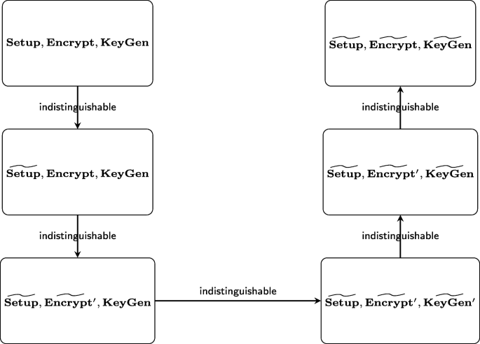

  

  Framework of Security Proof

  Table 1 Hybrid argument sequence with structure of ciphertexts and secret keys

• 2 Hybrid H₂: This experiment is the same as H₁ except that the master secret key and the public parameters are generated by $\widetilde {\mathbf {Setup}}$. Namely, the ciphertext ct_x and the secret key sk_y are generated by IPE.Encrypt and IPE.KeyGen:

  $$ ct_{\boldsymbol{x}}=\left(\boldsymbol{x},\alpha,0,\eta,0,0\right)_{\mathbb{B}},\ sk_{\boldsymbol{y}}=\left(\boldsymbol{y},0,\beta,0,\theta,0\right)_{\mathbb{B}^{*}}. $$

• 3 Hybrid H₃: This experiment is the same as H₂ except that every challenge ciphertext is $ct_{\boldsymbol {x}}=\left (\boldsymbol {x},\alpha,0,\eta,0,\gamma ^{\prime }\right)_{\mathbb {B}}$, which is generated by $\widetilde {\mathbf {Encrypt^{\prime }}}$.

• 4 Hybrid H₄: This experiment is the same as H₃ except that every challenge ciphertext is $ct_{\boldsymbol {x}}=\left (\boldsymbol {x},\alpha,0,0,0,\gamma ^{\prime }\right)_{\mathbb {B}}$, which is generated by $\widetilde {\mathbf {Encrypt}}$.

• 5 Hybrid H₅: This experiment is the same as H₄ except that, for every secret key query y, the corresponding secret key is $sk_{\boldsymbol {y}}=(\boldsymbol {y},0,\beta,\tau ^{\prime },\theta,0)_{\mathbb {B}^{*}}$, which is generated by $\widetilde {\mathbf {KeyGen^{\prime }}}$.

• 6 Hybrid H₆: This experiment is the same as H₅ except that, for every secret key query y, the corresponding secret key is $sk_{\boldsymbol {y}}=(\boldsymbol {y},0,\beta,\tau ^{\prime },0,0)_{\mathbb {B}^{*}}$, which is generated by $\widetilde {\mathbf {KeyGen}}$.

□

Lemma 7

For all PPT adversaries $\mathcal {A},\ \boldsymbol {H_1} \stackrel {c}{\approx } \boldsymbol {H_2}$.

Proof

Because the master secret key and the public parameters are all generated by IPE.Setup in H₁ and H₂, the view of $\mathcal {A}$ in H₁ and that in H₂ has the same distribution. □

Lemma 8

Assuming that Problem2 holds, for all PPT adversaries $\mathcal {A},\ \boldsymbol {H_2} \stackrel {c}{\approx } \boldsymbol {H_3}$.

Proof

Suppose that there exists a PPT adversary $\mathcal {A}$ that can distinguish the output distributions of H₂ and H₃. Then, we construct a PPT algorithm $\mathcal {B}$ which is given an instance of Problem2 $\left (\mathsf {param}_{\mathbb {V}},\widehat {\mathbb {B}},\widehat {\mathbb {B}}^{*},\boldsymbol {g}_{b}\right)$ for b∈{0,1} and simulates H₂ and H₃.

Setup:$\mathcal {B}$ runs IPE.Setup(1^λ,n) and outputs ${msk} = \left (\widehat {\mathbb {B}},\widehat {\mathbb {B}}^{*}\right)$ and ${pp} = \left (1^{\lambda }, \sf {param}_{\mathbb {V}}\right)$. $\mathcal {B}$ gives $\mathcal {A}$ the public parameters pp and the master secret key msk is only known to $\mathcal {B}$.

Secret Key Queries: To answer the key queries made by $\mathcal {A}, \mathcal {B}$ runs algorithm IPE.KeyGen to respond with $sk_{\boldsymbol {y}}=(\boldsymbol {y},0,\beta,0,\theta,0)_{\mathbb {B}^{*}}$.

Simulated Ciphertexts:$\mathcal {B}$ randomly chooses μ={1,⋯,q₁}, where q₁ is the number of the ciphertext queries asked by adversary $\mathcal {A}$. To answer the ciphertext query that $\mathcal {A}$ makes, $\mathcal {B}$ chooses $\alpha,\eta \stackrel {\sf {U}}{\leftarrow } \mathbb {Z}_{q}$ and $\gamma ^{\prime } \stackrel {\sf {U}}{\leftarrow } \mathbb {Z}_{q}^{\times }$ and computes ct_x as

$$\begin{array}{*{20}l} ct_{\boldsymbol{x}} &= \sum\limits_{l=1}^n x_l \boldsymbol{b}_l + \alpha \boldsymbol{b}_{n+1} + \eta \boldsymbol{b}_{n+3} + \gamma^{\prime} \boldsymbol{b}_{n+5} \text{if}\ l<\mu, \\ ct_{\boldsymbol{x}} &= \sum\limits_{l=1}^n x_l \boldsymbol{b}_l + \boldsymbol{g}_{b} \text{if}\ l=\mu, \\ ct_{\boldsymbol{x}} &= \sum\limits_{i=l}^n x_l \boldsymbol{b}_l + \alpha \boldsymbol{b}_{n+1} + \eta \boldsymbol{b}_{n+3} \text{if}\ l>\mu. \end{array} $$

We analyse that the view of $\mathcal {A}$ is composed of the public parameters and the answers of the secret key queries and the ciphertext queries. The public parameters in H₂ and H₃ are all generated by IPE.Setup and thus have the same distribution, similar to the answers to the secret key queries. It can be seen that if b=0, the answer is distributed as in H₂, if b=1, the answer is distributed as in H₃. □

Lemma 9

Assuming that Problem3 holds, for all PPT adversaries $\mathcal {A}, \boldsymbol {H_3} \stackrel {c}{\approx } \boldsymbol {H_4}$.

Proof

Suppose that there exists a PPT adversary $\mathcal {A}$ that can distinguish the output distributions of H₃ and H₄. Then, we construct a PPT algorithm $\mathcal {B}$ which is given an instance of Problem3 $\left (\mathsf {param}_{\mathbb {V}},\widehat {\mathbb {B}},\widehat {\mathbb {B}}^{*},\boldsymbol {g}_{b}\right)$ for b∈{0,1} and simulates H₃ and H₄.

Setup:$\mathcal {B}$ runs IPE.Setup(1^λ,n) and outputs ${msk} = \left (\widehat {\mathbb {B}},\widehat {\mathbb {B}}^{*}\right)$ and ${pp} = \left (1^{\lambda },\mathsf {param}_{\mathbb {V}}\right)$. $\mathcal {B}$ gives $\mathcal {A}$ the public parameters pp and the master secret key msk is only known to $\mathcal {B}$.

Secret Key Queries: To answer the key queries made by $\mathcal {A}, \mathcal {B}$ runs algorithm IPE.KeyGen to respond with $sk_{\boldsymbol {y}}=(\boldsymbol {y},0,\beta,0,\theta,0)_{\mathbb {B}^{*}}$.

Simulated Ciphertexts:$\mathcal {B}$ randomly chooses μ={1,⋯,q₁}, where q₁ is the number of the ciphertext queries asked by adversary $\mathcal {A}$. To answer the ciphertext query that $\mathcal {A}$ makes, $\mathcal {B}$ chooses random $\alpha, \eta \stackrel {\mathsf {U}}{\leftarrow } \mathbb {Z}_{q}$ and $\gamma ^{\prime } \stackrel {\mathsf {U}}{\leftarrow } \mathbb {Z}_{q}^{\times }$ and computes and answers as

$$\begin{array}{*{20}l} ct_{\boldsymbol{x}} &= \sum\limits_{l=1}^n x_l \boldsymbol{b}_l + \alpha \boldsymbol{b}_{n+1} + \gamma^{\prime} \boldsymbol{b}_{n+5} \text{if}\ l<\mu,\\ ct_{\boldsymbol{x}} &= \sum\limits_{l=1}^n x_l \boldsymbol{b}_l + \boldsymbol{g}_{b} \text{if}\ l=\mu,\\ ct_{\boldsymbol{x}} &= \sum\limits_{l=1}^n x_l \boldsymbol{b}_l + \alpha \boldsymbol{b}_{n+1} + \eta \boldsymbol{b}_{n+3} + \gamma^{\prime} \boldsymbol{b}_{n+5} \text{if}\ l>\mu.\\ \end{array} $$

We analyse that the view of $\mathcal {A}$ is composed of the public parameters and the answers of the secret key queries and the ciphertext queries. The public parameters in H₃ and H₄ are all generated by IPE.Setup and thus have the same distribution, similar to the answers to the secret key queries. It can be seen that if b=0, the answer is distributed as in H₃, if b=1, the answer is distributed as in H₄. □

Lemma 10

Assuming that Problem4 holds, for all PPT adversaries $\mathcal {A}, \boldsymbol {H_4} \stackrel {c}{\approx } \boldsymbol {H_5}$.

Proof

Suppose that there exists a PPT adversary $\mathcal {A}$ that can distinguish the output distributions of H₄ and H₅. Then, we construct a PPT algorithm $\mathcal {B}$ which is given an instance of Problem4 $\left (\mathsf {param}_{\mathbb {V}},\widehat {\mathbb {B}},\widehat {\mathbb {B}}^{*},\boldsymbol {g}_{b}^{*}\right)$ for b∈{0,1} and simulates H₄ and H₅.

Setup:$\mathcal {B}$ runs IPE.Setup(1^λ,n) and outputs ${msk} = \left (\widehat {\mathbb {B}},\widehat {\mathbb {B}}^{*}\right)$ and ${pp} = \left (1^{\lambda },\mathsf {param}_{\mathbb {V}}\right)$. $\mathcal {B}$ gives $\mathcal {A}$ the public parameters pp and the master secret key msk is only known to $\mathcal {B}$.

Ciphertexts Queries: To answer every ciphertext query that $\mathcal {A}$ makes, $\mathcal {B}$ chooses random $\alpha \stackrel {\mathsf {U}}{\leftarrow } \mathbb {Z}_{q}$ and $\gamma ^{\prime } \stackrel {\mathsf {U}}{\leftarrow } \mathbb {Z}_{q}^{\times }$, runs $\widetilde {\mathbf {Encrypt}}$, and answers as $ct_{\boldsymbol {x}}=(\boldsymbol {x},\alpha,0,0,0,\gamma ^{\prime })_{\mathbb {B}}$.

Simulated Secret Keys:$\mathcal {B}$ randomly chooses ν={1,⋯,q₂}, where q₂ is the number of the secret key queries asked by adversary $\mathcal {A}$. To answer the secret key query that $\mathcal {A}$ makes, $\mathcal {B}$ chooses $\beta,\theta \stackrel {\mathsf {U}}{\leftarrow } \mathbb {Z}_q$ and $\tau ^{\prime } \stackrel {\mathsf {U}}{\leftarrow } \mathbb {Z}_{q}^{\times }$ and computes and answers as

$$\begin{array}{*{20}l} sk_{\boldsymbol{y}} &= \sum\limits_{j=1}^n y_j \boldsymbol{b}_{j}^{*} + \beta \boldsymbol{b}_{n+2}^{*} + \tau^{\prime} \boldsymbol{b}_{n+3}^{*}+ \theta \boldsymbol{b}_{n+4}^{*} \text{if}\ j<\nu, \\ sk_{\boldsymbol{y}} &= \sum\limits_{j=1}^n y_j \boldsymbol{b}_{j}^{*} + \boldsymbol{g}_{b} \text{if}\ j=\nu, \\ sk_{\boldsymbol{y}} &= \sum\limits_{j=1}^n y_j \boldsymbol{b}_{j}^{*} + \beta \boldsymbol{b}_{n+2}^{*} + \theta \boldsymbol{b}_{n+4}^{*} \text{if}\ j>\nu. \\ \end{array} $$

We analyse that the view of $\mathcal {A}$ is composed of the public parameters and the answers of the ciphertexts queries and the secret key queries. The public parameters in H₄ and H₅ are all generated by IPE.Setup and thus have the same distribution, similar to the answers to ciphertexts queries where ct_x in H₄ and H₅ are all generated by $\widetilde {\mathbf {Encrypt}}$. It can be seen that if b=0, the answer is distributed as in H₄, if b=1, the answer is distributed as in H₅. □

Lemma 11

Assuming that Problem5 holds, for all PPT adversaries $\mathcal {A}, \boldsymbol {H_5} \stackrel {c}{\approx } \boldsymbol {H_6}$.

Proof

Suppose that there exists a PPT adversary $\mathcal {A}$ that can distinguish the output distributions of H₅ and H₆. Then, we construct a PPT algorithm $\mathcal {B}$ which is given an instance of Problem5 ($\mathsf {param}_{\mathbb {V}},\widehat {\mathbb {B}},\widehat {\mathbb {B}}^{*},\boldsymbol {g}_{b}^{*}$) for b∈{0,1} and simulates H₅ and H₆.

Setup:$\mathcal {B}$ runs IPE.Setup(1^λ,n) and outputs ${msk} = \left (\widehat {\mathbb {B}},\widehat {\mathbb {B}}^{*}\right)$ and ${pp} = \left (1^{\lambda },\sf {\mathsf {param}_{\mathbb {V}}}\right)$. $\mathcal {B}$ gives $\mathcal {A}$ the public parameters pp and the master secret key msk is only known to $\mathcal {B}$.

Ciphertexts Queries: To answer every ciphertext query that $\mathcal {A}$ makes, $\mathcal {B}$ chooses random $\alpha \stackrel {\mathsf {U}}{\leftarrow } \mathbb {Z}_{q}$ and $\gamma ^{\prime } \stackrel {\mathsf {U}}{\leftarrow } \mathbb {Z}_{q}^{\times }$, runs $\widetilde {\mathbf {Encrypt}}$, and answers as $ct_{\boldsymbol {x}}=(\boldsymbol {x},\alpha,0,0,0,\gamma ^{\prime })_{\mathbb {B}}$.

Simulated Secret Keys:$\mathcal {B}$ randomly chooses ν={1,⋯,q₂}, where q₂ is the number of the ciphertext queries asked by adversary $\mathcal {A}$. To answer the secret key query that $\mathcal {A}$ makes, $\mathcal {B}$ chooses $\beta,\theta \stackrel {\sf {U}}{\leftarrow } \mathbb {Z}_{q}$ and $\tau ^{\prime } \stackrel {\sf {U}}{\leftarrow } \mathbb {Z}_{q}^{\times }$ and computes and answers as

$$\begin{array}{*{20}l} sk_{\boldsymbol{y}} &= \sum\limits_{j=1}^n y_j \boldsymbol{b}_{j}^{*} + \beta \boldsymbol{b}_{n+2}^{*} + \tau^{\prime} \boldsymbol{b}_{n+3}^{*} + \text{if}\ j<\nu, \\ sk_{\boldsymbol{y}} &= \sum\limits_{j=1}^n y_j \boldsymbol{b}_{j}^{*} + \boldsymbol{g}_{b}^{*} \text{if}\ j=\nu, \\ sk_{\boldsymbol{y}} &= \sum\limits_{j=1}^n y_j \boldsymbol{b}_{j}^{*} + \beta \boldsymbol{b}_{n+2}^{*} + \tau^{\prime} \boldsymbol{b}_{n+3}^{*}+ \theta \boldsymbol{b}_{n+4}^{*} \text{if}\ j>\nu. \\ \end{array} $$

We analyse that the view of $\mathcal {A}$ is composed of the public parameters and the answers of the ciphertexts queries and the secret key queries. The public parameters in H₅ and H₆ are all generated by IPE.Setup and thus have the same distribution, similar to the answers to ciphertexts queries where ct_x in H₅ and H₆ are all generated by $\widetilde {\mathbf {Encrypt}}$. It can be seen that if b=0, the answer is distributed as in H₅, if b=1, the answer is distributed as in H₆. □

So we complete the proof.

Comparison

To demonstrate the advantage of our IPE scheme, we compare it with some related schemes (Bishop et al. 2015; Tomida et al. 2016; Datta et al. 2017; Zhao et al. 2018; Zhao et al. 2018) in the Table 2. Performance in our scheme is superior to that in the previous schemes in both storage complexity and computation complexity. Our scheme has shorter secret keys and ciphertexts. Additionally, our scheme is secure under weaker assumptions than other schemes. IND and SIM mean indistinguishability-based security and simulation-based security, respectively. KeyGen and Encrypt mean scalar multiplication on a cyclic group of IPE.KeyGen algorithm and IPE.Encrypt algorithm, respectively, and Decrypt means pairing operation on a bilinear pairing group of IPE.Decryption algorithm.

Table 2 Performance comparison of our IPE scheme

Conclusion

In this paper, we presented an efficient private-key inner product encryption scheme which achieves simulation-based security. Our scheme utilizes asymmetric bilinear pairing groups of prime order under the XDLIN assumption. There are still some open problems for inner product encryption can be explored and researched further. One of the problems is to build unbounded FE schemes for different functionalities, such as Quadratic Polynomials (Baltico et al. 2017). Another one is to construct a Multi-Input inner product encryption scheme under simulation-based security. Abdalla et al. (2017).

References

Abdalla, M, Bourse F, Caro AD, Pointcheval D (2015) Simple functional encryption schemes for inner products. In: Katz J (ed)Public-Key Cryptography - PKC 2015, 733–751.. Springer, Berlin.
Abdalla, M, Bourse F, Caro AD, Pointcheval D (2016) Better security for functional encryption for inner product evaluations. IACR Cryptol ePrint Arch 2016:11.
Abdalla, M, Gay R, Raykova M, Wee H (2017) Multi-input inner-product functional encryption from pairings In: Annual International Conference on the Theory and Applications of Cryptographic Techniques, 601–626.. Springer International Publishing, Cham.
Abe, M, Nishimaki R, Chase M, David B, Kohlweiss M, Ohkubo M (2016) Constant-size structure-preserving signatures: Generic constructions and simple assumptions. J Cryptol 29(4):833–878.
Agrawal, S, Agrawal S, Badrinarayanan S, Kumarasubramanian A, Prabhakaran M, Sahai A (2015) On the practical security of inner product functional encryption. Public-Key Cryptography – PKC 2015 :777–798.
Agrawal, S, Libert B, Maitra M, Titiu R (2020) Adaptive simulation security for inner product functional encryption. Public-Key Cryptography -PKC 2020 12110:34–64.
Agrawal, S, Libert B, Stehle D (2016) Fully secure functional encryption for inner products, from standard assumptions. Advances in Cryptology – CRYPTO 2016 :333–362.
Attrapadung, N, Libert B (2010) Functional encryption for inner product: Achieving constant-size ciphertexts with adaptive security or support for negation. In: Nguyen PQ Pointcheval D (eds)Public Key Cryptography – PKC 2010, 384–402.. Springer Berlin Heidelberg, Berlin.
Baltico, CEZ, Catalano D, Fiore D, Gay R (2017) Practical functional encryption for quadratic functions with applications to predicate encryption. Advances in Cryptology – CRYPTO 2017 :67–98.
Bishop, A, Jain A, Kowalczyk L (2015) Function-hiding inner product encryption In: Advances in Cryptology - ASIACRYPT 2015, 470–491.. Springer Berlin Heidelberg, Berlin.
Boneh, D, Franklin M (2001) Identity-based encryption from the weil pairing, 213–229.. Springer Berlin Heidelberg, Berlin.
Caro, AD, Iovino V, Jain A, O’Neill A, Paneth O, Persiano G (2013) On the achievability of simulation-based security for functional encryption. In: Canetti R Garay JA (eds)Advances in Cryptology – CRYPTO 2013, 519–535.. Springer Berlin Heidelberg, Berlin.
Caro, AD, Iovino V, Persiano G (2012) Fully secure hidden vector encryption In: Pairing-Based Cryptography - Paring 2012, 102–121.. Springer Berlin Heidelberg, Berlin.
Dan, B, Sahai A, Waters B (2011) Functional encryption: Definitions and challenges In: Theory of Cryptography Conference, 253–273.. Springer Berlin Heidelberg, Berlin.
Datta, P, Dutta R, Mukhopadhyay S (2016) Functional encryption for inner product with full function privacy. Public-Key Cryptography - PKC 2016:164–195.
Datta, P, Dutta R, Mukhopadhyay S (2017) Strongly full-hiding inner product encryption. Theor Comput Sci 667:16–50.
Datta, P, Okamoto T, Tomida J (2018) Full-hiding (unbounded) multi-input inner product functional encryption from the K-linear assumption In: Public-Key Cryptography, PKC 2018, 245–277.. Springer International Publishing, Cham.
Dufour-Sans, E, Pointcheval D (2019) Unbounded Inner-Product Functional Encryption with Succinct Keys. In: Deng RH, Gauthier-Umaña V, Ochoa M, Yung M (eds)Applied Cryptography and Network Security, 426–441.. Springer International Publishing, Cham.
Garg, S, Gentry C, Halevi S, Raykova M, Sahai A, Waters B (2016) Candidate indistinguishability obfuscation and functional encryption for all circuits. SIAM J Comput 45:882–929.
Goldwasser, S, Gordon SD, Goyal V, Jain A, Katz J, Liu F-H, Sahai A, Shi E, Zhou H-S (2014) Multi-input functional encryption. In: Nguyen PQ Oswald E (eds)Advances in Cryptology – EUROCRYPT 2014, 578–602.. Springer Berlin Heidelberg, Berlin.
Goyal, V, Pandey O, Sahai A, Waters B (2006) Attribute-based encryption for fine-grained access control of encrypted data In: Extended abstract to appear in ACM CCS 2006, 89–98.
Iovino, V, Persiano G (2008) Hidden-vector encryption with groups of prime order In: Pairing-Based Cryptography – Paring 2008, 75–88.. Springer Berlin Heidelberg, Berlin.
Katz, J, Sahai A, Waters B (2008) Predicate encryption supporting disjunctions, polynomial equations, and inner products. In: Smart N (ed)Advances in Cryptology – EUROCRYPT 2008, 146–162.. Springer, Berlin.
Kawai, Y, Takashima K (2013) Predicate- and attribute-hiding inner product encryption in a public key setting. Lect Notes Comput Sci 8365:113–130.
Kim, S, Kim J, Seo J (2019) A new approach to practical function-private inner product encryption. Theoretical Computer Science 783:22–40.
Kim, S, Lewi K, Mandal A, Montgomery H, Wu DJ (2018) Function-hiding inner product encryption is practical. In: Catalano D De Prisco R (eds)Security and Cryptography for Networks, 544–562.. Springer International Publishing, Cham.
Lewko, A, Okamoto T, Sahai A, Takashima K, Waters B (2010) Fully secure functional encryption: Attribute-based encryption and (hierarchical) inner product encryption. In: Gilbert H (ed)Advances in Cryptology – EUROCRYPT 2010, 62–91.. Springer, Berlin.
Okamoto, T (2011) Achieving short ciphertexts or short secret-keys for adaptively secure general inner product encryption. Cans 77(2-3):725–771.
Okamoto, T, Takashima K (2009) Hierarchical predicate encryption for inner-products In: International Conference on Advances in Cryptology–Asiacrypt, 214–231.. Springer Berlin Heidelberg, Berlin.
Okamoto, T, Takashima K (2012) Adaptively attribute-hiding (hierarchical) inner product encryption. In: Pointcheval D Johansson T (eds)Advances in Cryptology – EUROCRYPT 2012, 591–608.. Springer Berlin Heidelberg, Berlin.
Okamoto, T, Takashima K (2012) Fully secure unbounded inner-product and attribute-based encryption. In: Wang X Sako K (eds)Advances in Cryptology – ASIACRYPT 2012, 349–366.. Springer Berlin Heidelberg, Berlin.
Okamoto, T, Takashima K (2015) Dual pairing vector spaces and their applications. IEICE Trans Fundam Electron Commun Comput Sci E98.A(1):3–15.
O’Neill, A (2010) Definitional issues in functional encryption. IACR Cryptol ePrint Arch 2010:556.
Park, JH (2011) Inner-product encryption under standard assumptions. Des Codes Crypt 58:235–257.
Shen, E, Shi E, Waters B (2009) Predicate privacy in encryption systems In: Theory of Cryptography, 457–473.. Springer Berlin Heidelberg, Berlin.
Tomida, J, Abe M, Okamoto T (2016) Efficient functional encryption for inner-product values with full-hiding security. Information Security 9866:408–425.
Tomida, J, Takashima K (2018) Unbounded Inner Product Functional Encryption from Bilinear Maps. In: Peyrin T Galbraith S (eds)Advances in Cryptology – ASIACRYPT 2018, 609–639.. Springer International Publishing, Cham.
Zhang, Y, Li Y, Wang Y (2019) Efficient inner encryption for mobile clients with constrained computation capacity. Int J Innov Comput Inf Control 15(1):209–226.
Zhao, Q, Zeng Q, Liu X (2018) Improved construction for inner product functional encryption. Secur Commu Netw 2018:1–12.
Zhao, Q, Zeng Q, Liu X, Xu H (2018) Simulation-based security of function-hiding inner product encryption. Sci Chin Inf Sc 61(4):048102.
Zhenlin, T, Wei Z (2015) A predicate encryption scheme supporting multiparty cloud computation In: 2015 International Conference on Intelligent Networking and Collaborative Systems, 252–256.
Acknowledgements
We would like to thank the anonymous reviewers for detailed comments and useful feedback.
Funding
This work is supported by National Natural Science Foundation of China (61872152), the Major Program of Guangdong Basic and Applied Research (2019B030302008), and Science and Technology Program of Guangzhou (201902010081).
Author information
Authors and Affiliations
Contributions
The first author constructed the scheme with careful security proofs and wrote the manuscript. The second author reviewed the manuscript and checked the validity of the scheme and the security proofs. He also proofread the manuscript and corrected the grammar mistakes. The third and the fourth authors joined the discussion of the work and designed the whole figures and tables of the manuscript. All author(s) read and approved the final manuscript.
Corresponding author
Ethics declarations
Competing interests
The authors declare that they have no competing interests.
Additional information
Publisher’s Note
Springer Nature remains neutral with regard to jurisdictional claims in published maps and institutional affiliations.
Rights and permissions
Open Access This article is licensed under a Creative Commons Attribution 4.0 International License, which permits use, sharing, adaptation, distribution and reproduction in any medium or format, as long as you give appropriate credit to the original author(s) and the source, provide a link to the Creative Commons licence, and indicate if changes were made. The images or other third party material in this article are included in the article’s Creative Commons licence, unless indicated otherwise in a credit line to the material. If material is not included in the article’s Creative Commons licence and your intended use is not permitted by statutory regulation or exceeds the permitted use, you will need to obtain permission directly from the copyright holder. To view a copy of this licence, visit http://creativecommons.org/licenses/by/4.0/.
About this article
Cite this article
Liu, W., Huang, Q., Chen, X. et al. Efficient functional encryption for inner product with simulation-based security. Cybersecur 4, 2 (2021). https://doi.org/10.1186/s42400-020-00067-1
Received:
Accepted:
Published:
DOI: https://doi.org/10.1186/s42400-020-00067-1